目录
概述
Canny算法的历史年代久远,但它却是我目前接触的当中使用的最多的一种,它的好是好在哪里,为什么它在目前的研究当中被广泛使用?如果只停留在表面的调用上,我们并不能厚颜无耻的说我们已经是一个专家了,推导它的底层逻辑,是否能在我们以后的学习中为我们提供一些好的思路呢?我不知道,因为只有试过才知道。
最优边缘检测
Canny的目标是为了找到一个最优的边缘检测算法,最优边缘检测的含义如下:
(1)最优检测:算法能够尽可能多标识出图像的实际边缘,缺漏检测的真实边缘的概率和误差检测的非边缘的概率都尽可能的小。
(2)最优定位准则:检测到的边缘点要与实际的边缘点的位置要最近,或由于噪声影响引起的检测出的边缘偏离物体的真实边缘程度最小。
(3)检测点与边缘点一一对应:算子检测的边缘点要与实际边缘的点一一对应。
算法实现的步骤
1、灰度化与高斯滤波
将图像变为灰度图像,减少通道,高斯滤波的作用是平滑图像,减少噪声,不让Canny算法检测时,误认为是边缘,所以在一开始就使用这个高斯滤波来减少比较突出的地方,简单的来说,不合适的地方我们和谐掉。
2、计算图像的梯度和梯度方向
比如在灰度图像中它只有明暗的变化,当某个地方的强度变化比较的剧烈,那么它就会形成一个边缘。
3、非极大值抑制
经过上面的操作,我们只是对图像进行了一个增强,而并不是找到真正的边,这样我们就通过NMS(Non-maximum-supperession),将不是边缘的像素点去除掉。
4、双阈值筛选边缘
通常我们会给一个Threshold,比这个阈值大的就会被保留,但它也有些许缺点,它会让我们丢失一些细节的点。所以我们来设定一个阈值的边界(每个都尝试是最好的检验方式)。
5、利用滞后的边界跟踪
强边界与弱边界的效果相差较大,我们将与强边界相连的弱边界认为是边界,其他的弱边界则会被抑制。
6、在图像中跟踪边缘
这里会使用滞后阈值(包含高阈值、低阈值),比如图像中的重要边缘时连续的曲线,我们先采用一个较大的阈值,尽可能的将真实的边缘包含到,在逐渐的增加我们的低阈值,这样我们就可以实现一个跟踪,获得完整的曲线。
数学推导
高斯滤波会在水平方向与垂直方向呈现高斯分布,但高斯分布并不是高斯滤波,高斯滤波与高斯模糊是相同的。
高斯分布:
二维:
(2k+1)*(2k+1):
重要的是需要理解,高斯卷积核大小的选择将影响Canny检测器的性能:尺寸越大,检测器对噪声的敏感度越低,但是边缘检测的定位误差也将略有增加,一般采用5*5是一个比较不错的选择,这里选择的时候一定得是奇数。
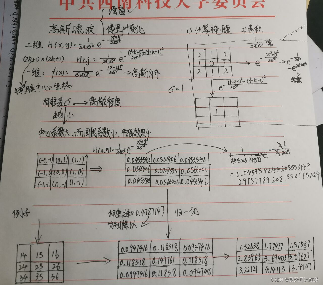
附带一张我的草稿图片,数学过程较多,再写到博客里就太麻烦了。
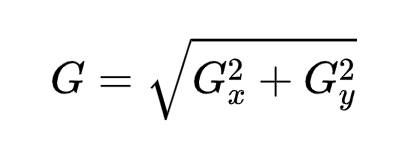
常见的方法采用Sobel滤波器(水平x和垂直y方向)在计算梯度和方向,水平方向Sobel算子Gx;用来检测y方向边缘,垂直方向Sobel算子Gy;用来检测x方向的边缘(边缘方向与梯度方向垂直)
求幅值公式:
求方位角公式: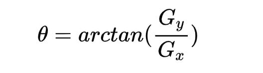
Opencv实现
import cv2
import numpy as np

def stackImages(scale,imgArray):
    rows = len(imgArray)
    cols = len(imgArray[0])
    rowsAvailable = isinstance(imgArray[0], list)
    width = imgArray[0][0].shape[1]
    height = imgArray[0][0].shape[0]
    if rowsAvailable:
        for x in range ( 0, rows):
            for y in range(0, cols):
                if imgArray[x][y].shape[:2] == imgArray[0][0].shape [:2]:
                    imgArray[x][y] = cv2.resize(imgArray[x][y], (0, 0), None, scale, scale)
                else:
                    imgArray[x][y] = cv2.resize(imgArray[x][y], (imgArray[0][0].shape[1], imgArray[0][0].shape[0]), None, scale, scale)
                if len(imgArray[x][y].shape) == 2: imgArray[x][y]= cv2.cvtColor( imgArray[x][y], cv2.COLOR_GRAY2BGR)
        imageBlank = np.zeros((height, width, 3), np.uint8)
        hor = [imageBlank]*rows
        hor_con = [imageBlank]*rows
        for x in range(0, rows):
            hor[x] = np.hstack(imgArray[x])
        ver = np.vstack(hor)
    else:
        for x in range(0, rows):
            if imgArray[x].shape[:2] == imgArray[0].shape[:2]:
                imgArray[x] = cv2.resize(imgArray[x], (0, 0), None, scale, scale)
            else:
                imgArray[x] = cv2.resize(imgArray[x], (imgArray[0].shape[1], imgArray[0].shape[0]), None,scale, scale)
            if len(imgArray[x].shape) == 2: imgArray[x] = cv2.cvtColor(imgArray[x], cv2.COLOR_GRAY2BGR)
        hor= np.hstack(imgArray)
        ver = hor
    return ver

img=cv2.imread("E:\pycharm\picture\\1-1-1.jpg")
img2=cv2.cvtColor(img,cv2.COLOR_BGR2GRAY)
img3=cv2.GaussianBlur(img2,(7,7),1)
img4=cv2.Canny(img3,50,180)
imgStack=stackImages(0.6,[img,img2,img3,img4])

cv2.imshow("Original_Grayscal_GuassianBlur_imgCanny",imgStack)
cv2.waitKey(0)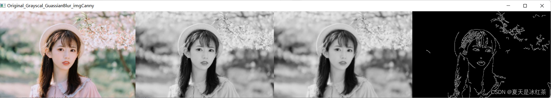
不要看我写这么长,其实主要的不是函数stackImage。
手写代码实现
(此代码来自于:Python实现Canny算子边缘检测 | Z Blog (yueyue200830.github.io))
import numpy as np
import cv2 as cv
from matplotlib import pyplot as plt
def smooth(image, sigma = 1.4, length = 5):
""" Smooth the image
Compute a gaussian filter with sigma = sigma and kernal_length = length.
Each element in the kernal can be computed as below:
G[i, j] = (1/(2*pi*sigma**2))*exp(-((i-k-1)**2 + (j-k-1)**2)/2*sigma**2)
Then, use the gaussian filter to smooth the input image.
Args:
image: array of grey image
sigma: the sigma of gaussian filter, default to be 1.4
length: the kernal length, default to be 5
Returns:
the smoothed image
"""
# Compute gaussian filter
k = length // 2
gaussian = np.zeros([length, length])
for i in range(length):
for j in range(length):
gaussian[i, j] = np.exp(-((i-k) ** 2 + (j-k) ** 2) / (2 * sigma ** 2))
gaussian /= 2 * np.pi * sigma ** 2
# Batch Normalization
gaussian = gaussian / np.sum(gaussian)
# Use Gaussian Filter
W, H = image.shape
new_image = np.zeros([W - k * 2, H - k * 2])
for i in range(W - 2 * k):
for j in range(H - 2 * k):
# 卷积运算
new_image[i, j] = np.sum(image[i:i+length, j:j+length] * gaussian)
new_image = np.uint8(new_image)
return new_image
def get_gradient_and_direction(image):
""" Compute gradients and its direction
Use Sobel filter to compute gradients and direction.
-1 0 1 -1 -2 -1
Gx = -2 0 2 Gy = 0 0 0
-1 0 1 1 2 1
Args:
image: array of grey image
Returns:
gradients: the gradients of each pixel
direction: the direction of the gradients of each pixel
"""
Gx = np.array([[-1, 0, 1], [-2, 0, 2], [-1, 0, 1]])
Gy = np.array([[-1, -2, -1], [0, 0, 0], [1, 2, 1]])
W, H = image.shape
gradients = np.zeros([W - 2, H - 2])
direction = np.zeros([W - 2, H - 2])
for i in range(W - 2):
for j in range(H - 2):
dx = np.sum(image[i:i+3, j:j+3] * Gx)
dy = np.sum(image[i:i+3, j:j+3] * Gy)
gradients[i, j] = np.sqrt(dx ** 2 + dy ** 2)
if dx == 0:
direction[i, j] = np.pi / 2
else:
direction[i, j] = np.arctan(dy / dx)
gradients = np.uint8(gradients)
return gradients, direction
def NMS(gradients, direction):
""" Non-maxima suppression
Args:
gradients: the gradients of each pixel
direction: the direction of the gradients of each pixel
Returns:
the output image
"""
W, H = gradients.shape
nms = np.copy(gradients[1:-1, 1:-1])
for i in range(1, W - 1):
for j in range(1, H - 1):
theta = direction[i, j]
weight = np.tan(theta)
if theta > np.pi / 4:
d1 = [0, 1]
d2 = [1, 1]
weight = 1 / weight
elif theta >= 0:
d1 = [1, 0]
d2 = [1, 1]
elif theta >= - np.pi / 4:
d1 = [1, 0]
d2 = [1, -1]
weight *= -1
else:
d1 = [0, -1]
d2 = [1, -1]
weight = -1 / weight
g1 = gradients[i + d1[0], j + d1[1]]
g2 = gradients[i + d2[0], j + d2[1]]
g3 = gradients[i - d1[0], j - d1[1]]
g4 = gradients[i - d2[0], j - d2[1]]
grade_count1 = g1 * weight + g2 * (1 - weight)
grade_count2 = g3 * weight + g4 * (1 - weight)
if grade_count1 > gradients[i, j] or grade_count2 > gradients[i, j]:
nms[i - 1, j - 1] = 0
return nms
def double_threshold(nms, threshold1, threshold2):
""" Double Threshold
Use two thresholds to compute the edge.
Args:
nms: the input image
threshold1: the low threshold
threshold2: the high threshold
Returns:
The binary image.
"""
visited = np.zeros_like(nms)
output_image = nms.copy()
W, H = output_image.shape
def dfs(i, j):
if i >= W or i < 0 or j >= H or j < 0 or visited[i, j] == 1:
return
visited[i, j] = 1
if output_image[i, j] > threshold1:
output_image[i, j] = 255
dfs(i-1, j-1)
dfs(i-1, j)
dfs(i-1, j+1)
dfs(i, j-1)
dfs(i, j+1)
dfs(i+1, j-1)
dfs(i+1, j)
dfs(i+1, j+1)
else:
output_image[i, j] = 0
for w in range(W):
for h in range(H):
if visited[w, h] == 1:
continue
if output_image[w, h] >= threshold2:
dfs(w, h)
elif output_image[w, h] <= threshold1:
output_image[w, h] = 0
visited[w, h] = 1
for w in range(W):
for h in range(H):
if visited[w, h] == 0:
output_image[w, h] = 0
return output_image
if __name__ == "__main__":
# code to read image
image = cv.imread('test.jpg',0)
cv.imshow("Original",image)
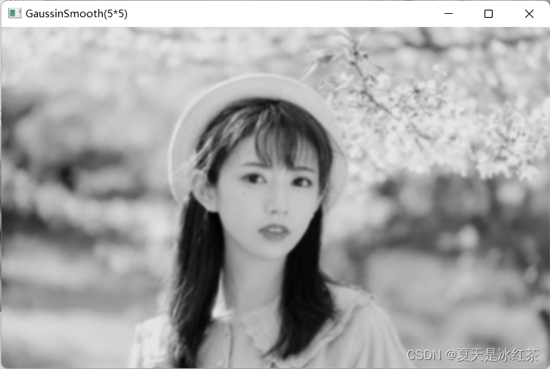
smoothed_image = smooth(image)
cv.imshow("GaussinSmooth(5*5)",smoothed_image)
gradients, direction = get_gradient_and_direction(smoothed_image)
# print(gradients)
# print(direction)
nms = NMS(gradients, direction)
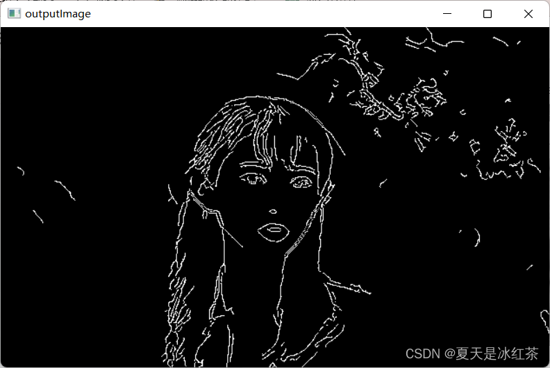
output_image = double_threshold(nms, 40, 100)
cv.imshow("outputImage",output_image)
cv.waitKey(0)
边缘检测定性分析
(以下皆为引用:一种基于改进Canny算法的图像边缘检测新方法)
将本文提出的新算法与现有几种经典边缘 5 检测算法对比分析,实验在 MATLAB R2018 a 的环境下进行。选取三类图像进数据仿真处理, 用 Prewitt 算法、Canny 算法、Sobel 算法、LoG 算法和本文算法进行实验,得到实验效果对比图。对 Lena 图像进行边缘检测得到图 2。

由图 2 可知,Sobel 算法和 Prewitt 算法检测的 边缘不全面不连续,但检测到的部分比较清晰。 LoG 算法能够检测到较为丰富的边缘,但对于噪 声不敏感且检测效果比较模糊。显然,本文算法 和经典 Canny 算法优于其它三种算法。经典 Canny 算法和本文改进的 Canny 算法在进行高斯滤波时 均选取相同的参数,边缘检测后,经典 Canny 算 法产生的伪边缘较多,本文算法相较经典 Canny 算法对于噪声不敏感,线条连续不杂乱。 选取电路板控制器图像,图像来源于文献 [1],来验证本文算法对于复杂图像的边缘检测 效果,得到图 3。
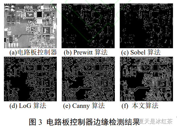
由图 3 对比看出,本文改进的 Canny 算法 能够保证边缘完整,同时检测边缘仍然清晰,具 有较好的图像检测效果。 为了验证本文算法的抗噪性能,对 rice 图像加入 0.05 的椒盐噪声,分别使用本文提到的五 种算法进行边缘检测,如图 4。
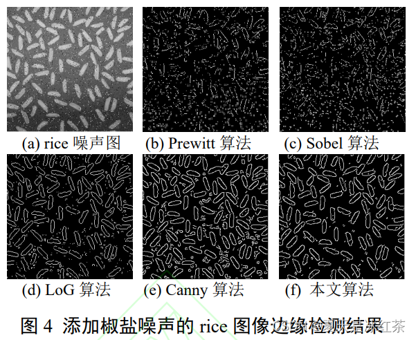
图 4 可以看出,Sobel 算法和 Prewitt 算法受 噪声影响很大,使图像边缘模糊,以至于几乎检 测不到边缘信息。LoG算法具有一定的抗噪性能, 但是边缘依旧模糊。本文算法和 Canny 算法明显 优于 Sobel 算法、Prewitt 算法和 LoG 算法。本文 算法检测的图像边缘完整准确,经典 Canny 算法 也能够提取出比较完整的图像边缘,但受噪声影 响比较大,出现了一些连续的噪声轮廓。
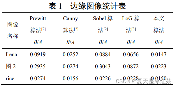
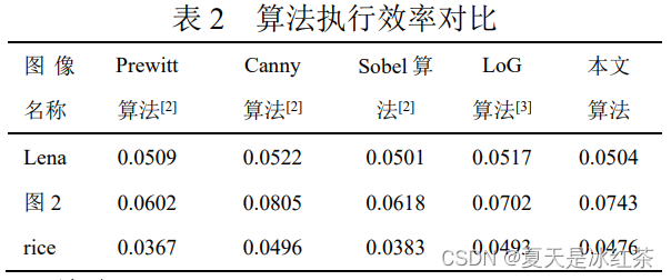
对五种算法执行效率进行对比,实验数据如 表 2,表 2 中的数据是五种算法 100 次边缘检测 实验取得的平均值。由统计数据得出,本文改进 的 Canny 算法的检测效率与 LoG 算法和经典 Canny 算法相近。