在本文中,我将和大家一起学习将使用机器学习数据集使用基本的探索性数据分析技术分析航班票价预测,然后根据某些特征(例如航空公司的类型、到达时间)得出一些关于航班价格的预测时间,出发时间,飞行时间,来源,目的地等等。
完整代码、技术交流,文末获取
写在前面
在本文中,我们使用机器学习进行预测,得出以下结论:
-
EDA: 了解EDA的完整流程
-
数据分析: 学会在数据集中从数学和可视化等上面获得一些见解。
-
数据可视化: 可视化数据方便挖掘更加直观的结论。
-
特征工程: 将在特征工程部分挖掘我们可以做的工作。
-
机器学习模型:学习做一个经过数据预处理等步骤的机器学习模型。
-
比较模型:将研究多个模型,并选择最佳模型。
关于数据集
-
Airline航空公司: 因此,本列将包含所有类型的航空公司,例如 Indigo、Jet Airways、Air India 等等。
-
Date_of_Journey旅程日期: 此列将告知我们乘客旅程的开始日期。
扫描二维码关注公众号,回复: 14448411 查看本文章
-
Source来源: 此列包含乘客旅程开始的地点名称。
-
Destination目的地: 此列包含乘客想要前往的地点的名称。
-
Route路线: 乘客选择从他/她的来源到目的地的路线是什么。
-
Arrival_Time到达时间: 到达时间是乘客到达目的地的时间。
-
Duration持续时间: 持续时间是航班完成从源头到目的地的旅程的整个时间。
-
Total_Stops停留总数: 航班在整个旅程中将在多少地方停留。
-
Additional_Info附加信息: 在此列有关食物、食物种类和其他便利设施的信息。
-
Price价格: 完整旅程的航班价格,包括登机前的所有费用。
导入库
import numpy as np
import pandas as pd

import matplotlib.pyplot as plt
import seaborn as sns

from sklearn.preprocessing import StandardScaler
from sklearn.model_selection import train_test_split
from sklearn.metrics import mean_squared_error as mse
from sklearn.metrics import r2_score
from math import sqrt
from sklearn.linear_model import Ridge
from sklearn.linear_model import Lasso
from sklearn.tree import DecisionTreeRegressor
from sklearn.ensemble import RandomForestRegressor
from sklearn.preprocessing import LabelEncoder
from sklearn.model_selection import KFold
from sklearn.model_selection import train_test_split
from sklearn.model_selection import GridSearchCV
from sklearn.model_selection import RandomizedSearchCV

from prettytable import PrettyTable
探索性数据分析 (EDA)
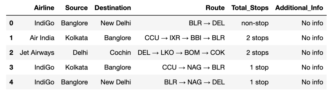
训练数据集
读取数据集的训练数据
train_df = pd.read_excel("Data_Train.xlsx")# 数据获取:在公众号:数据STUDIO 后台回复 data
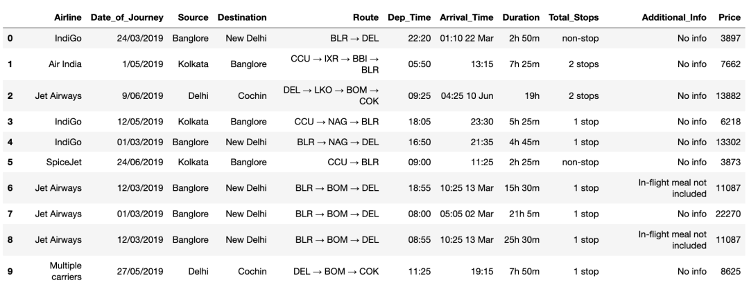
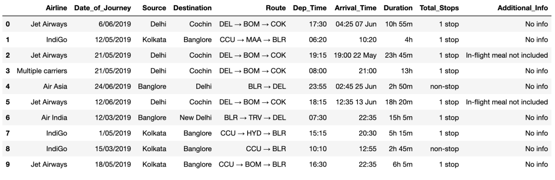
train_df.head(10)
如果你的文件特别大,建议使用如下方法读取。
> import datatable as dt
> train_df = dt.fread("Data_Train.xlsx").to_pandas()
查看数据信息
现在查看数据集所具有的列类型
train_df.columns
Index(['Airline', 'Date_of_Journey', 'Source',
       'Destination', 'Route', 'Dep_Time',
       'Arrival_Time', 'Duration', 'Total_Stops',
       'Additional_Info', 'Price'],
      dtype='object')
在这里,我们可以获得有关我们的数据集的更多信息
train_df.info()
<class 'pandas.core.frame.DataFrame'>
RangeIndex: 10683 entries, 0 to 10682
Data columns (total 11 columns):
 #   Column           Non-Null Count  Dtype
---  ------           --------------  -----
 0   Airline          10683 non-null  object
 1   Date_of_Journey  10683 non-null  object
 2   Source           10683 non-null  object
 3   Destination      10683 non-null  object
 4   Route            10682 non-null  object
 5   Dep_Time         10683 non-null  object
 6   Arrival_Time     10683 non-null  object
 7   Duration         10683 non-null  object
 8   Total_Stops      10682 non-null  object
 9   Additional_Info  10683 non-null  object
 10  Price            10683 non-null  int64
dtypes: int64(1), object(10)
memory usage: 918.2+ KB
描述性统计
了解有关数据集的更多信息
train_df.describe()
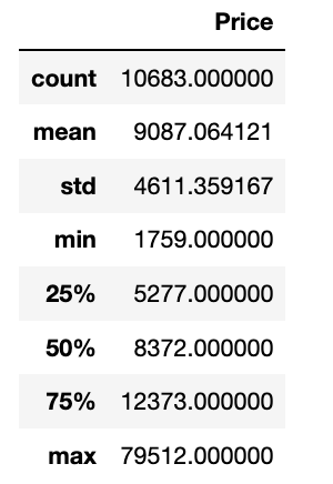
因为只有价格是数值型变量,因此描述性统计只能输出该结果。
缺失值统计
使用 isnull 函数时,看到数据集中是否是空值的信息
train_df.isnull().head()
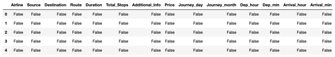
使用 isnull 函数和 sum 函数时,看到数据集中空值的数量
train_df.isnull().sum()
Airline            0
Date_of_Journey    0
Source             0
Destination        0
Route              1
Dep_Time           0
Arrival_Time       0
Duration           0
Total_Stops        1
Additional_Info    0
Price              0
dtype: int64
删除缺失值值
train_df.dropna(inplace=True)
重复值
train_df[train_df.duplicated()].head()
从数据集中删除那些重复的值
train_df.drop_duplicates(keep='first',inplace=True)
分析各个变量信息
检查 Additional_info 列并计算唯一类型的值。
train_df["Additional_Info"].value_counts()
No info                         8182
In-flight meal not included     1926
No check-in baggage included     318
1 Long layover                    19
Change airports                    7
Business class                     4
No Info                            3
1 Short layover                    1
2 Long layover                     1
Red-eye flight                     1
Name: Additional_Info, dtype: int64
检查不同的航空公司
train_df["Airline"].unique()
array(['IndiGo', 'Air India', 'Jet Airways',
       'SpiceJet', 'Multiple carriers', 'GoAir',
       'Vistara', 'Air Asia', 'Vistara Premium economy',
       'Jet Airways Business', 'Trujet',
       'Multiple carriers Premium economy'],
       dtype=object)
检查不同的航线。
train_df["Route"].unique()
上下滑动查看更多
array(['BLR → DEL', 'CCU → IXR → BBI → BLR', 'DEL → LKO → BOM → COK',
       'CCU → NAG → BLR', 'BLR → NAG → DEL', 'CCU → BLR',
       'BLR → BOM → DEL', 'DEL → BOM → COK', 'DEL → BLR → COK',
       'MAA → CCU', 'CCU → BOM → BLR', 'DEL → AMD → BOM → COK',
       'DEL → PNQ → COK', 'DEL → CCU → BOM → COK', 'BLR → COK → DEL',
       'DEL → IDR → BOM → COK', 'DEL → LKO → COK',
       'CCU → GAU → DEL → BLR', 'DEL → NAG → BOM → COK',
       'CCU → MAA → BLR', 'DEL → HYD → COK', 'CCU → HYD → BLR',
       'DEL → COK', 'CCU → DEL → BLR', 'BLR → BOM → AMD → DEL',
       'BOM → DEL → HYD', 'DEL → MAA → COK', 'BOM → HYD',
       'DEL → BHO → BOM → COK', 'DEL → JAI → BOM → COK',
       'DEL → ATQ → BOM → COK', 'DEL → JDH → BOM → COK',
       'CCU → BBI → BOM → BLR', 'BLR → MAA → DEL',
       'DEL → GOI → BOM → COK', 'DEL → BDQ → BOM → COK',
       'CCU → JAI → BOM → BLR', 'CCU → BBI → BLR', 'BLR → HYD → DEL',
       'DEL → TRV → COK', 'CCU → IXR → DEL → BLR',
       'DEL → IXU → BOM → COK', 'CCU → IXB → BLR',
       'BLR → BOM → JDH → DEL', 'DEL → UDR → BOM → COK',
       'DEL → HYD → MAA → COK', 'CCU → BOM → COK → BLR',
       'BLR → CCU → DEL', 'CCU → BOM → GOI → BLR',
       'DEL → RPR → NAG → BOM → COK', 'DEL → HYD → BOM → COK',
       'CCU → DEL → AMD → BLR', 'CCU → PNQ → BLR',
       'BLR → CCU → GAU → DEL', 'CCU → DEL → COK → BLR',
       'BLR → PNQ → DEL', 'BOM → JDH → DEL → HYD',
       'BLR → BOM → BHO → DEL', 'DEL → AMD → COK', 'BLR → LKO → DEL',
       'CCU → GAU → BLR', 'BOM → GOI → HYD', 'CCU → BOM → AMD → BLR',
       'CCU → BBI → IXR → DEL → BLR', 'DEL → DED → BOM → COK',
       'DEL → MAA → BOM → COK', 'BLR → AMD → DEL', 'BLR → VGA → DEL',
       'CCU → JAI → DEL → BLR', 'CCU → AMD → BLR',
       'CCU → VNS → DEL → BLR', 'BLR → BOM → IDR → DEL',
       'BLR → BBI → DEL', 'BLR → GOI → DEL', 'BOM → AMD → ISK → HYD',
       'BOM → DED → DEL → HYD', 'DEL → IXC → BOM → COK',
       'CCU → PAT → BLR', 'BLR → CCU → BBI → DEL',
       'CCU → BBI → HYD → BLR', 'BLR → BOM → NAG → DEL',
       'BLR → CCU → BBI → HYD → DEL', 'BLR → GAU → DEL',
       'BOM → BHO → DEL → HYD', 'BOM → JLR → HYD',
       'BLR → HYD → VGA → DEL', 'CCU → KNU → BLR',
       'CCU → BOM → PNQ → BLR', 'DEL → BBI → COK',
       'BLR → VGA → HYD → DEL', 'BOM → JDH → JAI → DEL → HYD',
       'DEL → GWL → IDR → BOM → COK', 'CCU → RPR → HYD → BLR',
       'CCU → VTZ → BLR', 'CCU → DEL → VGA → BLR',
       'BLR → BOM → IDR → GWL → DEL', 'CCU → DEL → COK → TRV → BLR',
       'BOM → COK → MAA → HYD', 'BOM → NDC → HYD', 'BLR → BDQ → DEL',
       'CCU → BOM → TRV → BLR', 'CCU → BOM → HBX → BLR',
       'BOM → BDQ → DEL → HYD', 'BOM → CCU → HYD',
       'BLR → TRV → COK → DEL', 'BLR → IDR → DEL',
       'CCU → IXZ → MAA → BLR', 'CCU → GAU → IMF → DEL → BLR',
       'BOM → GOI → PNQ → HYD', 'BOM → BLR → CCU → BBI → HYD',
       'BOM → MAA → HYD', 'BLR → BOM → UDR → DEL',
       'BOM → UDR → DEL → HYD', 'BLR → VGA → VTZ → DEL',
       'BLR → HBX → BOM → BHO → DEL', 'CCU → IXA → BLR',
       'BOM → RPR → VTZ → HYD', 'BLR → HBX → BOM → AMD → DEL',
       'BOM → IDR → DEL → HYD', 'BOM → BLR → HYD', 'BLR → STV → DEL',
       'CCU → IXB → DEL → BLR', 'BOM → JAI → DEL → HYD',
       'BOM → VNS → DEL → HYD', 'BLR → HBX → BOM → NAG → DEL',
       'BLR → BOM → IXC → DEL', 'BLR → CCU → BBI → HYD → VGA → DEL',
       'BOM → BBI → HYD'], dtype=object)
测试数据集
test_df = pd.read_excel("Test_set.xlsx")
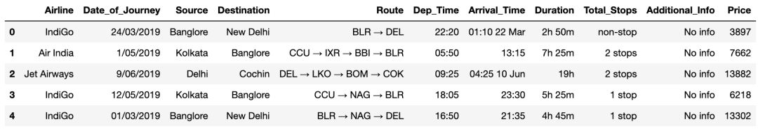
test_df.head(10)
查看测试数据所具有的列类型。
test_df.columns
Index(['Airline', 'Date_of_Journey', 'Source',
        'Destination', 'Route', 'Dep_Time',
        'Arrival_Time', 'Duration', 'Total_Stops',
       'Additional_Info'],
      dtype='object')
有关数据集的信息。
test_df.info()
<class 'pandas.core.frame.DataFrame'>
RangeIndex: 2671 entries, 0 to 2670
Data columns (total 10 columns):
 #   Column           Non-Null Count  Dtype
---  ------           --------------  -----
 0   Airline          2671 non-null   object
 1   Date_of_Journey  2671 non-null   object
 2   Source           2671 non-null   object
 3   Destination      2671 non-null   object
 4   Route            2671 non-null   object
 5   Dep_Time         2671 non-null   object
 6   Arrival_Time     2671 non-null   object
 7   Duration         2671 non-null   object
 8   Total_Stops      2671 non-null   object
 9   Additional_Info  2671 non-null   object
dtypes: object(10)
memory usage: 208.8+ KB
了解有关测试数据集的更多信息。
test_df.describe()
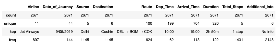
这里注意下,训练集和测试集使用同一个方法,得到的结果确不同。这是因为描述性统计中describe函数优先对数值型数据进行分析统计,当输入数据中没有数值型数据时,则会对非数值型数据进行分析统计。因此会得到count、unique、top、freq等针对非数值型变量进行统计信息。
使用 isnull 函数和 sum 函数,得到测试数据中空值的数量。
test_df.isnull().sum()
Airline            0
Date_of_Journey    0
Source             0
Destination        0
Route              0
Dep_Time           0
Arrival_Time       0
Duration           0
Total_Stops        0
Additional_Info    0
dtype: int64
特征工程
查看处理过的数据
train_df.head()
将小时转换为分钟
train_df['Duration'] = train_df['Duration']\
           .str.replace("h", '*60')\
           .str.replace(' ','+')\
           .str.replace('m','*1')\
           .apply(eval)
test_df['Duration'] = test_df['Duration']\
                      .str.replace("h", '*60')\
                      .str.replace(' ','+')\
                      .str.replace('m','*1')\
                      .apply(eval)
Date_of_Journey:
在数据集中组织旅程日期的格式,以便在模型阶段进行更好的预处理。
# Date_of_Journey
train_df["Journey_day"] = train_df['Date_of_Journey'].str.split('/').str[0].astype(int)
train_df["Journey_month"] = train_df['Date_of_Journey'].str.split('/').str[1].astype(int)
train_df.drop(["Date_of_Journey"], axis = 1, inplace = True)
Dep_Time:
将出发时间转换为小时和分钟。
# Dep_Time
train_df["Dep_hour"] = pd.to_datetime(train_df["Dep_Time"]).dt.hour
train_df["Dep_min"] = pd.to_datetime(train_df["Dep_Time"]).dt.minute
train_df.drop(["Dep_Time"], axis = 1, inplace = True)
Arrival_Time:
同样,将到达时间转换为小时和分钟。
# Arrival_Time
train_df["Arrival_hour"] = pd.to_datetime(train_df.Arrival_Time).dt.hour
train_df["Arrival_min"] = pd.to_datetime(train_df.Arrival_Time).dt.minute
train_df.drop(["Arrival_Time"], axis = 1, inplace = True)
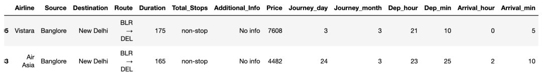
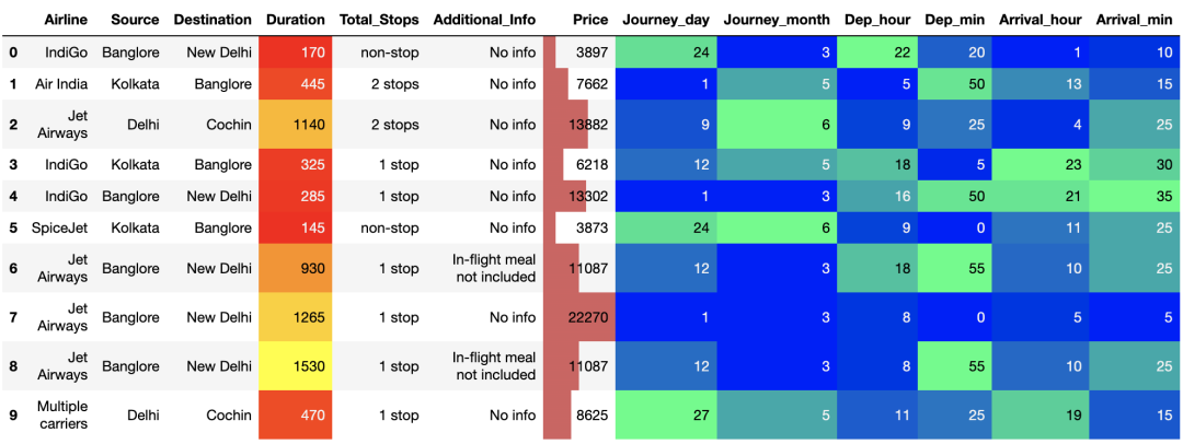
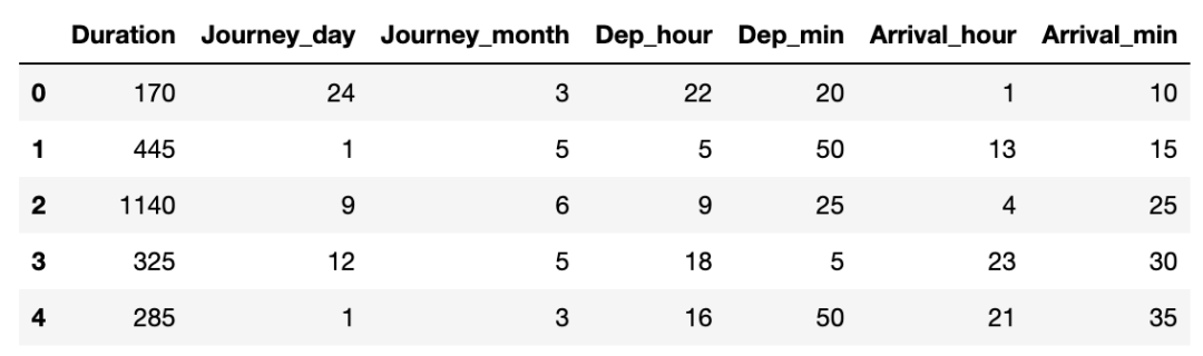
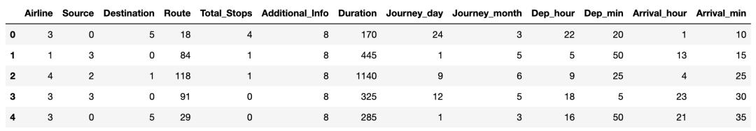
现在在最后的预处理之后让我们看看我们的数据集。
train_df.head(10).style.hide(axis='columns',subset=['Route'])\
                       .background_gradient(subset=['Journey_day','Journey_month','Dep_hour',
                                                  'Dep_min','Arrival_hour','Arrival_min']
                                         ,cmap='winter')\
                        .background_gradient(subset=['Duration'], cmap='autumn')\
                    .bar(subset=['Price'])
数据可视化
绘制价格与航空公司图
g = sns.catplot(y = "Price",
                x = "Airline",
                data = train_df.sort_values(
                    "Price",
                    ascending = False),
                kind="boxen",
                height = 8,
                aspect = 3,
                ax=ax)
add_name(g.ax) # 添加水印文字
g.fig.set_dpi(150)

推论: 在这里,借助catplot图,绘制航班价格和航空公司价格之间的箱线图,可以得出结论,Jet Airways 在价格方面的异常值最多。
绘制价格与来源的小提琴图
g = sns.catplot(y = "Price",
                x = "Source",
                data = train_df.sort_values(
                    "Price",
                    ascending = False),
                kind="violin",
                height = 4,
                aspect = 3)
add_name(g.ax)
g.fig.set_dpi(150)

推论: 现在仅借助catplot图,在航班价格和出发地之间绘制箱线图,即乘客将从哪里前往目的地,可以看到作为出发地的Banglore具有最多异常值,而Chennai最少。
绘制价格与目的地的箱线图
g = sns.catplot(y = "Price",
                x = "Destination",
                data = train_df.sort_values(
                    "Price",
                    ascending = False),
                kind="box", height = 4,
                aspect = 3)
add_name(g.ax)
g.fig.set_dpi(150)
plt.show()

推论: 在这里,在航班价格和乘客旅行目的地之间的catplot图的帮助下绘制箱线图,并发现New Delhi的异常值最多,Kolkata的异常值最少。
绘制月份(持续时间)与航班数量的条形图
plt.figure(figsize = (10, 5),dpi=150)
plt.title('Count of flights month wise')
ax=sns.countplot(x = 'Journey_month', data = train_df)
plt.xlabel('Month')
plt.ylabel('Count of flights')
for p in ax.patches:
    ax.annotate(int(p.get_height()),
                   (p.get_x()+0.25,
                   p.get_height()+1),
                   va='bottom',
                   color= 'black')
推论: 在上图中,我们绘制了一个月旅程与几个航班的计数图,并看到五月的航班数量最多。
绘制航空公司类型与航班数量的条形图
plt.figure(figsize = (20,5),dpi=200)
plt.title('不同航空公司的航班数')
ax=sns.countplot(x = 'Airline', data =train_df)
plt.xlabel('航空公司')
plt.ylabel('航班数')
plt.xticks(rotation = 30)
for p in ax.patches:
    ax.annotate(int(p.get_height()),
                   (p.get_x()+0.25,
                    p.get_height()+1),
                va='bottom', color= 'black')
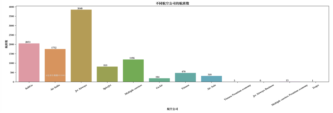
推论: 现在从上图航空公司类型和航班数量之间比较中可以看到,Jet Airways 登机的航班最多。
绘制机票价格 VS 航空公司
plt.figure(figsize = (15,4),dpi=200)
plt.title('价格 VS 航空公司')
plt.scatter(train_df['Airline'],
            train_df['Price'])
plt.xticks
plt.xlabel('航空公司')
plt.ylabel('票价')
plt.xticks(rotation = 30)
特征相关性分析
绘制相关性
plt.figure(figsize = (15,15))
sns.heatmap(train_df.corr(),
            annot = True,
            cmap = "RdYlGn")
plt.show()

删除Price列
因为它是目标变量
data = train_df.drop(["Price"], axis=1)
处理分类数据和数值数据
train_categorical_data = data.select_dtypes(exclude=['int64', 'float','int32'])
train_numerical_data = data.select_dtypes(include=['int64', 'float','int32'])

test_categorical_data = test_df.select_dtypes(exclude=['int64', 'float','int32','int32'])
test_numerical_data = test_df.select_dtypes(include=['int64', 'float','int32'])
train_categorical_data.head()
train_numerical_data.head()
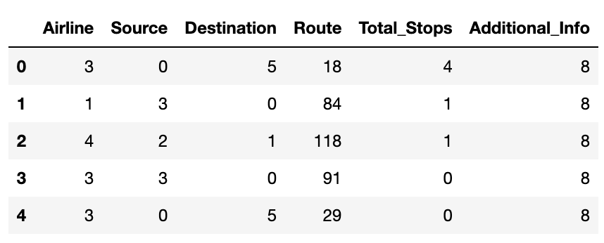
分类列的标签编码和热编码
le = LabelEncoder()
train_categorical_data = train_categorical_data.apply(LabelEncoder().fit_transform)
test_categorical_data = test_categorical_data.apply(LabelEncoder().fit_transform)
train_categorical_data.head()
连接分类数据和数值数据
X = pd.concat([train_categorical_data, train_numerical_data], axis=1)
y = train_df['Price']
test_set = pd.concat([test_categorical_data, test_numerical_data], axis=1)
X.head()
y.head()
0     3897
1     7662
2    13882
3     6218
4    13302
Name: Price, dtype: int32
机器学习模型
如上文所演示,我们已经完成了一个完整的 EDA 流程,获得了数据分析、特征工程和数据可视化,因此在所有这些步骤之后,我们可以使用机器学习模型制作步骤进行预测。
划分训练集和测试集
X_train, X_test, y_train, y_test = train_test_split(
      X, y, test_size = 0.3, random_state = 42)

print("训练集输入大小", X_train.shape)
print("训练集输出大小", y_train.shape)
print("测试集输入大小", X_test.shape)
print("测试集输出大小", y_test.shape)
训练集输入大小 (7477, 13)
训练集输出大小 (7477,)
测试集输入大小 (3205, 13)
测试集输出大小 (3205,)
模型构建
Ridge Regression
执行GridSearchCV岭回归。
params = {

    'alpha' : [0.0001, 0.001, 0.01, 0.1, 1, 10, 100, 1000, 10000, 100000]}
ridge_regressor = GridSearchCV(Ridge(), params, cv = 5,
                               scoring = 'neg_mean_absolute_error',
                               n_jobs = -1)
ridge_regressor.fit(X_train, y_train)
GridSearchCV(cv=5, estimator=Ridge(), n_jobs=-1,
             param_grid={

    'alpha': [0.0001, 0.001, 0.01, 0.1, 1, 10, 100, 1000,
                                   10000, 100000]},
             scoring='neg_mean_absolute_error')
定义计算平均绝对百分比误差的函数。
def mean_absolute_percentage_error(y_true, y_pred):
    y_true, y_pred = np.array(y_true), np.array(y_pred)
    return np.mean(np.abs((y_true - y_pred) / y_true)) * 100
预测训练和测试结果。
y_train_pred = ridge_regressor.predict(X_train)
y_test_pred = ridge_regressor.predict(X_test)
打印模型评估结果。
print("Train Results for Ridge Regressor Model:")
print("Root Mean Squared Error: ", sqrt(mse(y_train.values, y_train_pred)))
print("Mean Absolute % Error: ", round(mean_absolute_percentage_error(y_train.values, y_train_pred)))
print("R-Squared: ", r2_score(y_train.values, y_train_pred))
Train Results for Ridge Regressor Model:
Root Mean Squared Error:  3558.667750232805
Mean Absolute % Error:  32
R-Squared:  0.4150529285926381
print("Test Results for Ridge Regressor Model:")
print("Root Mean Squared Error: ", sqrt(mse(y_test, y_test_pred)))
print("Mean Absolute % Error: ", round(mean_absolute_percentage_error(y_test, y_test_pred)))
print("R-Squared: ", r2_score(y_test, y_test_pred))
Test Results for Ridge Regressor Model:
Root Mean Squared Error:  3457.5985597925214
Mean Absolute % Error:  32
R-Squared:  0.42437171409958274
Lasso Regression
执行GridSearchCV套索回归。
params = {

    'alpha' : [0.0001, 0.001, 0.01, 0.1, 1, 10, 100, 1000, 10000, 100000]}
lasso_regressor = GridSearchCV(Lasso(), params , cv = 15,
                               scoring = 'neg_mean_absolute_error',
                               n_jobs = -1)
lasso_regressor.fit(X_train, y_train)
GridSearchCV(cv=15, estimator=Lasso(), n_jobs=-1,
             param_grid={

    'alpha': [0.0001, 0.001, 0.01, 0.1, 1, 10, 100, 1000,
                                   10000, 100000]},
             scoring='neg_mean_absolute_error')
预测训练和测试结果。
y_train_pred = lasso_regressor.predict(X_train)
y_test_pred = lasso_regressor.predict(X_test)
打印模型评估结果。
print("Train Results for Lasso Regressor Model:")
print("Root Mean Squared Error: ", sqrt(mse(y_train.values, y_train_pred)))
print("Mean Absolute % Error: ", round(mean_absolute_percentage_error(y_train.values, y_train_pred)))
print("R-Squared: ", r2_score(y_train.values, y_train_pred))
Train Results for Lasso Regressor Model:
Root Mean Squared Error:  3560.853987663486
Mean Absolute % Error:  32
R-Squared:  0.4143339932536655
print("Test Results for Lasso Regressor Model:")
print("Root Mean Squared Error: ", sqrt(mse(y_test, y_test_pred)))
print("Mean Absolute % Error: ", round(mean_absolute_percentage_error(y_test, y_test_pred)))
print("R-Squared: ", r2_score(y_test, y_test_pred))
Test Results for Lasso Regressor Model:
Root Mean squared Error:  3459.384927631988
Mean Absolute % Error:  32
R-Squared:  0.4237767638929625
Decision Tree Regression
执行GridSearchCV决策树回归。
depth = list(range(3,30))
param_grid = dict(max_depth = depth)
tree = GridSearchCV(DecisionTreeRegressor(), param_grid, cv = 10)
tree.fit(X_train,y_train)
预测训练和测试结果。
y_train_pred = tree.predict(X_train)
y_test_pred = tree.predict(X_test)
打印模型评估结果。
print("Train Results for Decision Tree Regressor Model:")
print("Root Mean Squared Error: ", sqrt(mse(y_train.values, y_train_pred)))
print("Mean Absolute % Error: ", round(mean_absolute_percentage_error(y_train.values, y_train_pred)))
print("R-Squared: ", r2_score(y_train.values, y_train_pred))
Train Results for Decision Tree Regressor Model:
Root Mean squared Error:  560.9099093439073
Mean Absolute % Error:  3
R-Squared:  0.9854679156224377
print("Test Results for Decision Tree Regressor Model:")
print("Root Mean Squared Error: ", sqrt(mse(y_test, y_test_pred)))
print("Mean Absolute % Error: ", round(mean_absolute_percentage_error(y_test, y_test_pred)))
print("R-Squared: ", r2_score(y_test, y_test_pred))
Test Results for Decision Tree Regressor Model:
Root Mean Squared Error:  1871.5387049259973
Mean Absolute % Error:  9
R-Squared:  0.8313483417949448
比较所有模型
ridge_score = round(ridge_regressor.score(X_train, y_train) * 100, 2)
ridge_score_test = round(ridge_regressor.score(X_test, y_test) * 100, 2)

lasso_score = round(lasso_regressor.score(X_train, y_train) * 100, 2)
lasso_score_test = round(lasso_regressor.score(X_test, y_test) * 100, 2)

decision_score = round(tree.score(X_train, y_train) * 100, 2)
decision_score_test = round(tree.score(X_test, y_test) * 100, 2)
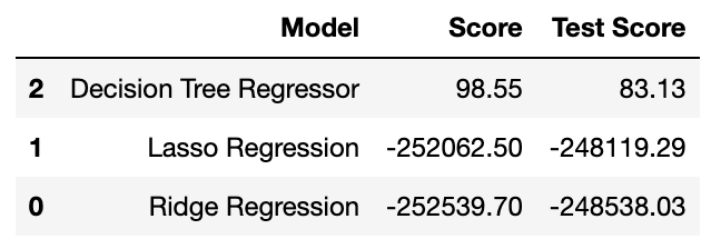
现在将本文中演示的三个模型进行比较。
models = pd.DataFrame({


    'Model': [ 'Ridge Regression', 'Lasso Regression','Decision Tree Regressor'],
    'Score': [ ridge_score, lasso_score, decision_score],
    'Test Score': [ ridge_score_test, lasso_score_test, decision_score_test]})
models.sort_values(by='Test Score', ascending=False)
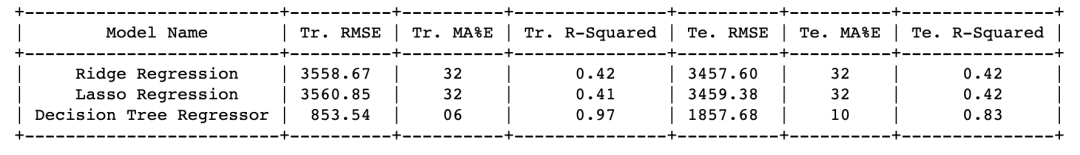
x.field_names = ["Model Name", "Tr. RMSE", "Tr. MA%E",
                 "Tr. R-Squared", "Te. RMSE", "Te. MA%E", "Te. R-Squared",]
x.add_row(['Ridge Regression','3558.67','32','0.42','3457.60','32','0.42'])
x.add_row(['Lasso Regression','3560.85','32','0.41','3459.38','32','0.42'])
x.add_row(['Decision Tree Regressor','853.54','06','0.97','1857.68','10','0.83'])
print(x)
总结
通过比较所有的模型(岭回归、套索回归、决策树回归),我们可以得出决策树回归性能最好。
联系方式
目前开通了技术交流群,群友已超过3000人,添加时最好的备注方式为:来源+兴趣方向,方便找到志同道合的朋友,资料、代码获取也可以加入
方式1、添加微信号:dkl88191,备注:来自CSDN
方式2、微信搜索公众号:Python学习与数据挖掘,后台回复:加群