此示例说明如何测量信号的相似性。它将帮助回答诸如以下的问题:如何比较具有不同长度或不同采样率的信号?如何在测量中发现存在信号还是只存在噪声?两个信号是否相关?如何测量两个信号之间的延迟(以及如何对齐它们)?如何比较两个信号的频率成分?也可以在信号的不同段中寻找相似性以确定信号是否为周期性信号。
比较具有不同采样率的信号
假设有一个音频信号数据库和一个模式匹配应用程序,需要在歌曲播放时识别该歌曲。数据通常以低采样率存储,以占用更少的内存。
load relatedsig.mat

figure
ax(1) = subplot(3,1,1);
plot((0:numel(T1)-1)/Fs1,T1,'k')
ylabel('Template 1')
grid on
ax(2) = subplot(3,1,2);
plot((0:numel(T2)-1)/Fs2,T2,'r')
ylabel('Template 2')
grid on
ax(3) = subplot(3,1,3);
plot((0:numel(S)-1)/Fs,S)
ylabel('Signal')
grid on
xlabel('Time (secs)')
linkaxes(ax(1:3),'x')
axis([0 1.61 -4 4])
如图所示:
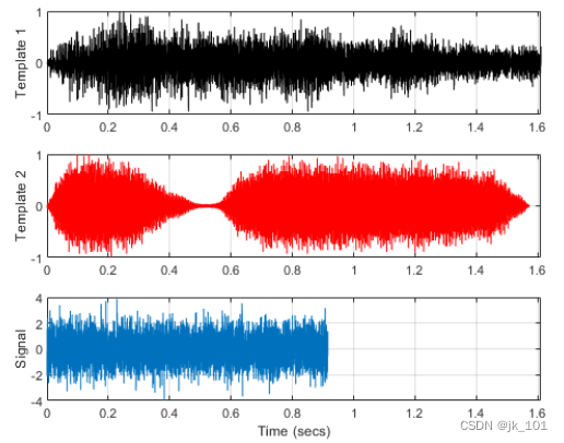
第一个和第二个子图显示来自数据库的模板信号。第三个子图显示我们要在数据库中搜索的信号。仅仅通过观察时间序列,该信号似乎与两个模板信号都不匹配。但仔细检查就会发现,这些信号实际上有不同的长度和采样率。
[Fs1 Fs2 Fs]


ans = 1×3

        4096        4096        8192
长度不同无法计算两个信号之间的差,但这可以通过提取信号的共同部分来轻松解决。此外,并不始终需要对长度进行均衡化处理。不同长度的信号之间可以执行互相关,但必须确保它们具有相同的采样率。最安全的做法是以较低的采样率对信号进行重采样。resample 函数在重采样过程中对信号应用一个抗混叠(低通)FIR 滤波器。
[P1,Q1] = rat(Fs/Fs1);          % Rational fraction approximation
[P2,Q2] = rat(Fs/Fs2);          % Rational fraction approximation
T1 = resample(T1,P1,Q1);        % Change sampling rate by rational factor
T2 = resample(T2,P2,Q2);        % Change sampling rate by rational factor
在测量中寻找信号
现在,我们可以使用 xcorr 函数将信号S 与模板 T1 和 T2 进行互相关,以确定是否存在匹配。
[C1,lag1] = xcorr(T1,S);
[C2,lag2] = xcorr(T2,S);

figure
ax(1) = subplot(2,1,1);
plot(lag1/Fs,C1,'k')
ylabel('Amplitude')
grid on
title('Cross-correlation between Template 1 and Signal')
ax(2) = subplot(2,1,2);
plot(lag2/Fs,C2,'r')
ylabel('Amplitude')
grid on
title('Cross-correlation between Template 2 and Signal')
xlabel('Time(secs)')
axis(ax(1:2),[-1.5 1.5 -700 700 ])
如图所示:

第一个子图指示信号和模板 1 的相关性较低,而第二个子图中的高峰值指示信号存在于第二个模板中。
[~,I] = max(abs(C2));
SampleDiff = lag2(I)

SampleDiff = 499

%%
timeDiff = SampleDiff/Fs

timeDiff = 0.0609
互相关峰值意味着信号在 61 毫秒后开始出现在模板 T2 中。换句话说,如 SampleDiff 所示,信号 T2 相对于信号 S 领先 499 个采样。此信息可用于对齐信号。
测量信号之间的延迟并将其对齐
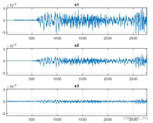
假设要从不同的传感器采集数据,记录桥两边的汽车引起的振动。当分析信号时,可能需要对齐它们。假设有 3 个传感器以相同的采样率工作,并且它们正在测量由同一事件引起的信号。
figure
ax(1) = subplot(3,1,1);
plot(s1)
ylabel('s1')
grid on
ax(2) = subplot(3,1,2);
plot(s2,'k')
ylabel('s2')
grid on
ax(3) = subplot(3,1,3);
plot(s3,'r')
ylabel('s3')
grid on
xlabel('Samples')
linkaxes(ax,'xy')
如图所示:

我们还可以使用finddelay 函数来找到两个信号之间的延迟。
t21 = finddelay(s1,s2)

t21 = -350

%%
t31 = finddelay(s1,s3)

t31 = 150
t21 表示 s2 相对于 s1 滞后 350 个采样,t31 表示 s3 相对于 s1 领先 150 个采样。现在可使用此信息通过时移信号来对齐这 3 个信号。我们也可以直接使用 alignsignals 函数来对齐信号,该函数通过延迟最早的信号来对齐两个信号。
s1 = alignsignals(s1,s3);
s2 = alignsignals(s2,s3);

figure
ax(1) = subplot(3,1,1);
plot(s1)
grid on
title('s1')
axis tight
ax(2) = subplot(3,1,2);
plot(s2)
grid on
title('s2')
axis tight
ax(3) = subplot(3,1,3);
plot(s3)
grid on
title('s3')
axis tight
linkaxes(ax,'xy')
如图所示:
比较信号的频率成分
功率谱显示每个频率中存在的功率。频谱相干性确定信号之间的频域相关性。趋向于 0 的相干性值表示对应的频率分量不相关,而趋向于 1 的值表示对应的频率分量相关。假设有两个信号,它们各自的功率谱如下。
Fs = FsSig;         % Sampling Rate

[P1,f1] = periodogram(sig1,[],[],Fs,'power');
[P2,f2] = periodogram(sig2,[],[],Fs,'power');

figure
t = (0:numel(sig1)-1)/Fs;
subplot(2,2,1)
plot(t,sig1,'k')
ylabel('s1')
grid on
title('Time Series')
subplot(2,2,3)
plot(t,sig2)
ylabel('s2')
grid on
xlabel('Time (secs)')
subplot(2,2,2)
plot(f1,P1,'k')
ylabel('P1')
grid on
axis tight
title('Power Spectrum')
subplot(2,2,4)
plot(f2,P2)
ylabel('P2')
grid on
axis tight
xlabel('Frequency (Hz)')
如图所示:

mscohere 函数计算两个信号之间的频谱相干性。它确认 sig1 和 sig2 在 35 Hz 和 165 Hz 附近有两个相关分量。在频谱相干性高的频率中,相关分量之间的相对相位可以用交叉频谱相位来估计。
[Cxy,f] = mscohere(sig1,sig2,[],[],[],Fs);
Pxy = cpsd(sig1,sig2,[],[],[],Fs);
phase = -angle(Pxy)/pi*180;
[pks,locs] = findpeaks(Cxy,'MinPeakHeight',0.75);

figure
subplot(2,1,1)
plot(f,Cxy)
title('Coherence Estimate')
grid on
hgca = gca;
hgca.XTick = f(locs);
hgca.YTick = 0.75;
axis([0 200 0 1])
subplot(2,1,2)
plot(f,phase)
title('Cross-spectrum Phase (deg)')
grid on
hgca = gca;
hgca.XTick = f(locs);
hgca.YTick = round(phase(locs));
xlabel('Frequency (Hz)')
axis([0 200 -180 180])
如图所示:
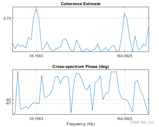
35 Hz 分量之间的相位滞后接近 -90 度,165 Hz 分量之间的相位滞后接近 -60 度。
求信号的周期性
假设存在一组冬季办公楼的温度测量值。测量每 30 分钟进行一次,持续约 16.5 周。
load officetemp.mat

Fs = 1/(60*30);                 % Sample rate is 1 sample every 30 minutes
days = (0:length(temp)-1)/(Fs*60*60*24);

figure
plot(days,temp)
title('Temperature Data')
xlabel('Time (days)')
ylabel('Temperature (Fahrenheit)')
grid on
如图所示:
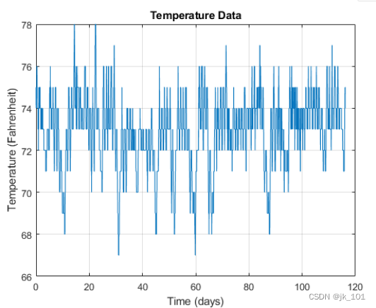
对于低于 70 度的温度,需要去除均值来分析信号中的微小波动。xcov 函数在计算互相关性之前去除信号的均值。它返回互协方差。将最大滞后限制为信号的 50%,以获得互协方差的良好估计值。
maxlags = numel(temp)*0.5;
[xc,lag] = xcov(temp,maxlags);

[~,df] = findpeaks(xc,'MinPeakDistance',5*2*24);
[~,mf] = findpeaks(xc);

figure
plot(lag/(2*24),xc,'k',...
     lag(df)/(2*24),xc(df),'kv','MarkerFaceColor','r')
grid on
xlim([-15 15])
xlabel('Time (days)')
title('Auto-covariance')
如图所示:
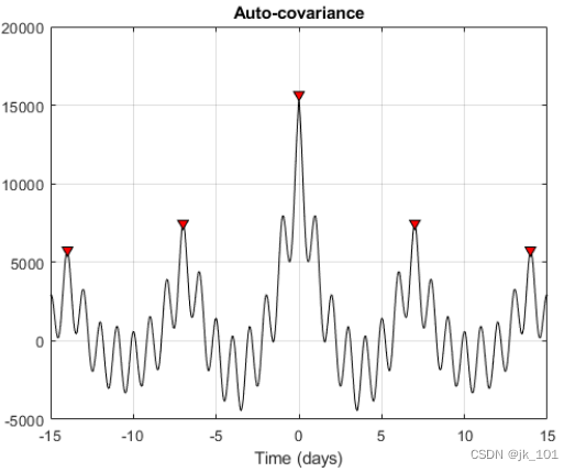
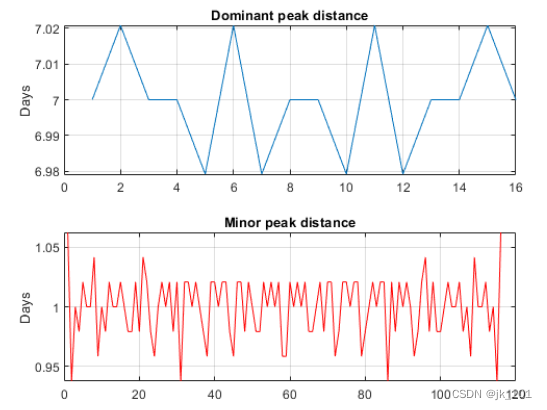
观察自协方差的主要和次要波动。主峰和次峰看起来是等距的。为了验证它们是否等距,请计算并绘制后续各峰值位置之间的差。
cycle1 = diff(df)/(2*24);
cycle2 = diff(mf)/(2*24);

subplot(2,1,1)
plot(cycle1)
ylabel('Days')
grid on
title('Dominant peak distance')
subplot(2,1,2)
plot(cycle2,'r')
ylabel('Days')
grid on
title('Minor peak distance')
如图所示:
mean(cycle1)

ans = 7


mean(cycle2)

ans = 1
次峰指示每周有 7 个周期,主峰指示每周有 1 个周期。这是合理的,因为数据来自以 7 天为日历周期的温控建筑物。第一个 7 天周期表明,建筑物温度存在以周为单位的周期行为,其中温度在周末较低,在工作日期间恢复正常。以 1 天为单位的周期行为表明还存在日周期行为 - 夜间温度降低,白天温度升高。