一、概述

对于机器学习模型，会考虑完整的像素方向，而不仅仅是数字。毕竟，机器学习模型是矩阵。因此，这些权重矩阵的值是根据输入数据的完整像素方向形成的。

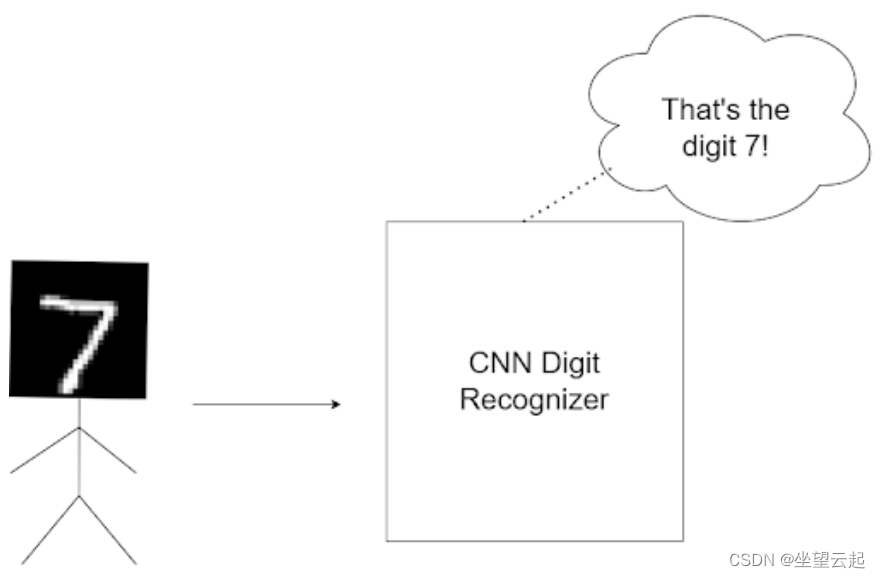
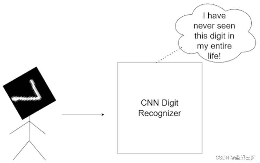
比如下面两个图像，对于没有旋转的数字，CNN预测正确，图像旋转之后可能预测就失败了，说明CNN不是旋转不变的，这在简单的测试或者实验中可能不是什么大问题，但是现实世界的不确定性因素导致在现实中应用的时候可能会遇到很多问题。

深度学习领域的快速研究人员已经提出了一个解决方案，即 Spatial Transformer Networks。

Spatial Transformer 网络模块背后的主要目的是帮助我们的模型选择最相关的图像 ROI。一旦模型成功计算出相关像素，空间变换模块将帮助模型决定图像需要什么样的变换才能成为标准格式。

模型必须找出一种转换，使其能够预测图像的正确标签。这可能不是我们可以理解的转换，但只要可以降低损失函数，它就适用于模型。

创建了整个模块，以便模型可以根据情况访问各种转换：平移、裁剪、各向同性和倾斜。您将在下一节中了解有关它的更多信息。

将空间变压器模块视为您模型的附加附件。它根据输入要求在前向传递期间将特定的空间变换应用于特征图。所以对于一个特定的输入，我们有一个输出特征图。

它将帮助我们的模型决定像图 2中的 7 这样的输入需要什么样的转换。对于多通道输入（例如，RGB 图像），相同的更改应用于所有三个通道（以保持空间一致性）。最重要的是，这个模块将与其他模型权重一起学习（它是可微的）。

显示了空间变换器模块，分为三个部分：定位网络、网格生成器和采样器。

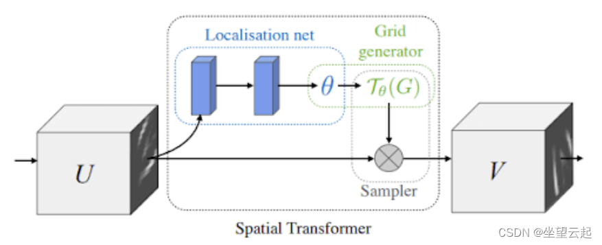
定位网络：该网络接受宽度为 W、高度为 H 和通道 C的输入特征图U。它的工作是输出 $\theta$ ，要应用于特征图的变换参数。定位网络可以是任何东西：全连接网络或卷积网络。

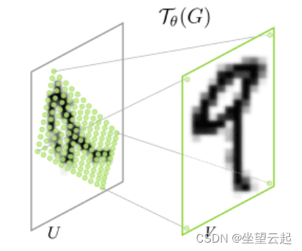
参数化采样网格：我们有转换的参数 $\theta$ . 假设我们的输入特征图是 U，如图 4所示。我们可以看到 U 是数字 9 的旋转版本。我们的输出特征图 V 是正方形网格。因此我们已经知道它的索引（即，一个普通的矩形网格）。

采样器：现在我们有了坐标，输出特征图 V 值将仅使用我们的输入像素值进行估计。也就是说，我们将使用输入像素对输出像素执行线性/双线性插值。双线性插值使用最近的像素值，这些像素值位于给定位置的对角线方向，以便找到该像素的适当颜色强度值。

二、创建配置文件

# import the necessary packages
from tensorflow.data import AUTOTUNE
import os
# define AUTOTUNE
AUTO = AUTOTUNE
# define the image height, width and channel size
IMAGE_HEIGHT = 28
IMAGE_WIDTH = 28
CHANNEL = 1
# define the dataset path, dataset name, and the batch size
DATASET_PATH = "dataset"
DATASET_NAME = "emnist"
BATCH_SIZE = 1024
# define the number of epochs
EPOCHS = 100
# define the conv filters
FILTERS = 256
# define an output directory
OUTPUT_PATH = "output"
# define the loss function and optimizer
LOSS_FN = "sparse_categorical_crossentropy"
OPTIMIZER = "adam"
# define the name of the gif
GIF_NAME = "stn.gif"
# define the number of classes for classification
CLASSES = 62
# define the stn layer name
STN_LAYER_NAME = "stn"

三、为输出 GIF 创建回调函数

这个函数将帮助我们构建我们的 GIF。它还允许我们在训练时跟踪模型的进度。

# import the necessary packages
from tensorflow.keras.callbacks import Callback
from tensorflow.keras import Model
import matplotlib.pyplot as plt
def get_train_monitor(testDs, outputPath, stnLayerName):
	# iterate over the test dataset and take a batch of test images
	(testImg, _) = next(iter(testDs))
	# define a training monitor
	class TrainMonitor(Callback):
		def on_epoch_end(self, epoch, logs=None):
			model = Model(self.model.input,
				self.model.get_layer(stnLayerName).output)
			testPred = model(testImg)
			# plot the image and the transformed image
			_, axes = plt.subplots(nrows=5, ncols=2, figsize=(5, 10))
			for ax, im, t_im  in zip(axes, testImg[:5], testPred[:5]):
				ax[0].imshow(im[..., 0], cmap="gray")
				ax[0].set_title(epoch)
				ax[0].axis("off")
				ax[1].imshow(t_im[..., 0], cmap="gray")
				ax[1].set_title(epoch)
				ax[1].axis("off")
			
			# save the figures
			plt.savefig(f"{outputPath}/{epoch:03d}")
			plt.close()
	
	# instantiate the training monitor callback
	trainMonitor = TrainMonitor()
	# return the training monitor object
	return trainMonitor

四、Spatial Transformer 模块

为了将空间转换器模块附加到我们的主模型，我们创建一个单独的脚本，其中包含所有必要的辅助函数以及主层。

输入图像将为我们提供所需的转换参数。
从输出特征图映射输入特征图。
应用双线性插值来估计输出特征图像素值。

# import the necessary packages
from tensorflow.keras import Sequential
from tensorflow.keras.layers import Conv2D
from tensorflow.keras.layers import MaxPool2D
from tensorflow.keras.layers import GlobalAveragePooling2D
from tensorflow.keras.layers import Reshape
from tensorflow.keras.layers import Dense
from tensorflow.keras.layers import Layer
import tensorflow as tf
def get_pixel_value(B, H, W, featureMap, x, y):
	# create batch indices and reshape it
	batchIdx = tf.range(0, B)
	batchIdx = tf.reshape(batchIdx, (B, 1, 1))
	# create the indices matrix which will be used to sample the 
	# feature map
	b = tf.tile(batchIdx, (1, H, W))
	indices = tf.stack([b, y, x], 3)
	# gather the feature map values for the corresponding indices
	gatheredPixelValue = tf.gather_nd(featureMap, indices)
	# return the gather pixel values
	return gatheredPixelValue

def affine_grid_generator(B, H, W, theta):
	# create normalized 2D grid
	x = tf.linspace(-1.0, 1.0, H)
	y = tf.linspace(-1.0, 1.0, W)
	(xT, yT) = tf.meshgrid(x, y)
	# flatten the meshgrid
	xTFlat = tf.reshape(xT, [-1])
	yTFlat = tf.reshape(yT, [-1])
	# reshape the meshgrid and concatenate ones to convert it to 
	# homogeneous form
	ones = tf.ones_like(xTFlat)
	samplingGrid = tf.stack([xTFlat, yTFlat, ones])
	# repeat grid batch size times
	samplingGrid = tf.broadcast_to(samplingGrid, (B, 3, H * W))
	# cast the affine parameters and sampling grid to float32 
	# required for matmul
	theta = tf.cast(theta, "float32")
	samplingGrid = tf.cast(samplingGrid, "float32")
	# transform the sampling grid with the affine parameter
	batchGrids = tf.matmul(theta, samplingGrid)
	# reshape the sampling grid to (B, H, W, 2)
	batchGrids = tf.reshape(batchGrids, [B, 2, H, W])
	# return the transformed grid
	return batchGrids

def bilinear_sampler(B, H, W, featureMap, x, y):
	# define the bounds of the image
	maxY = tf.cast(H - 1, "int32")
	maxX = tf.cast(W - 1, "int32")
	zero = tf.zeros([], dtype="int32")
	# rescale x and y to feature spatial dimensions
	x = tf.cast(x, "float32")
	y = tf.cast(y, "float32")
	x = 0.5 * ((x + 1.0) * tf.cast(maxX-1, "float32"))
	y = 0.5 * ((y + 1.0) * tf.cast(maxY-1, "float32"))
	# grab 4 nearest corner points for each (x, y)
	x0 = tf.cast(tf.floor(x), "int32")
	x1 = x0 + 1
	y0 = tf.cast(tf.floor(y), "int32")
	y1 = y0 + 1
	# clip to range to not violate feature map boundaries
	x0 = tf.clip_by_value(x0, zero, maxX)
	x1 = tf.clip_by_value(x1, zero, maxX)
	y0 = tf.clip_by_value(y0, zero, maxY)
	y1 = tf.clip_by_value(y1, zero, maxY)
	# get pixel value at corner coords
	Ia = get_pixel_value(B, H, W, featureMap, x0, y0)
	Ib = get_pixel_value(B, H, W, featureMap, x0, y1)
	Ic = get_pixel_value(B, H, W, featureMap, x1, y0)
	Id = get_pixel_value(B, H, W, featureMap, x1, y1)
	# recast as float for delta calculation
	x0 = tf.cast(x0, "float32")
	x1 = tf.cast(x1, "float32")
	y0 = tf.cast(y0, "float32")
	y1 = tf.cast(y1, "float32")
	# calculate deltas
	wa = (x1-x) * (y1-y)
	wb = (x1-x) * (y-y0)
	wc = (x-x0) * (y1-y)
	wd = (x-x0) * (y-y0)
	# add dimension for addition
	wa = tf.expand_dims(wa, axis=3)
	wb = tf.expand_dims(wb, axis=3)
	wc = tf.expand_dims(wc, axis=3)
	wd = tf.expand_dims(wd, axis=3)
	# compute transformed feature map
	transformedFeatureMap = tf.add_n(
		[wa * Ia, wb * Ib, wc * Ic, wd * Id])
	# return the transformed feature map
	return transformedFeatureMap

class STN(Layer):
	def __init__(self, name, filter):
		# initialize the layer
		super().__init__(name=name)
		self.B = None
		self.H = None
		self.W = None
		self.C = None
		# create the constant bias initializer
		self.output_bias = tf.keras.initializers.Constant(
			[1.0, 0.0, 0.0,
			0.0, 1.0, 0.0]
		)
		# define the filter size
		self.filter = filter

	def build(self, input_shape):
		# get the batch size, height, width and channel size of the
		# input
		(self.B, self.H, self.W, self.C) = input_shape
		# define the localization network
		self.localizationNet = Sequential([
			Conv2D(filters=self.filter // 4, kernel_size=3,
				input_shape=(self.H, self.W, self.C), 
				activation="relu", kernel_initializer="he_normal"),
			MaxPool2D(),
			Conv2D(filters=self.filter // 2, kernel_size=3,
				activation="relu", kernel_initializer="he_normal"),
			MaxPool2D(),
			Conv2D(filters=self.filter, kernel_size=3,
				activation="relu", kernel_initializer="he_normal"),
			MaxPool2D(),
			GlobalAveragePooling2D()
		])
		# define the regressor network
		self.regressorNet = tf.keras.Sequential([
			Dense(units = self.filter, activation="relu",
				kernel_initializer="he_normal"),
			Dense(units = self.filter // 2, activation="relu",
				kernel_initializer="he_normal"),
			Dense(units = 3 * 2, kernel_initializer="zeros",
				bias_initializer=self.output_bias),
			Reshape(target_shape=(2, 3))
		])

	def call(self, x):
		# get the localization feature map
		localFeatureMap = self.localizationNet(x)
		# get the regressed parameters
		theta = self.regressorNet(localFeatureMap)
		# get the transformed meshgrid
		grid = affine_grid_generator(self.B, self.H, self.W, theta)
		# get the x and y coordinates from the transformed meshgrid
		xS = grid[:, 0, :, :]
		yS = grid[:, 1, :, :]
		# get the transformed feature map
		x = bilinear_sampler(self.B, self.H, self.W, x, xS, yS)
		# return the transformed feature map
		return x

五、创建分类模型

# import the necessary packages
from tensorflow.keras import Input
from tensorflow.keras import Model
from tensorflow.keras.layers import Conv2D
from tensorflow.keras.layers import MaxPool2D
from tensorflow.keras.layers import Reshape
from tensorflow.keras.layers import GlobalAveragePooling2D
from tensorflow.keras.layers import Lambda
from tensorflow.keras.layers import Dense
from tensorflow.keras.layers import Dropout
import tensorflow as tf
def get_training_model(batchSize, height, width, channel, stnLayer,
	numClasses, filter):
	# define the input layer and pass the input through the STN
	# layer
	inputs = Input((height, width, channel), batch_size=batchSize)
	x = Lambda(lambda image: tf.cast(image, "float32")/255.0)(inputs)
	x = stnLayer(x) 

	# apply a series of conv and maxpool layers
	x = Conv2D(filter // 4, 3, activation="relu", 
		kernel_initializer="he_normal")(x)
	x = MaxPool2D()(x)
	x = Conv2D(filter // 2, 3, activation="relu",
		kernel_initializer="he_normal")(x)
	x = MaxPool2D()(x)
	x = Conv2D(filter, 3, activation="relu",
		kernel_initializer="he_normal")(x)
	x = MaxPool2D()(x)
	# global average pool the output of the previous layer
	x = GlobalAveragePooling2D()(x)
	# pass the flattened output through a couple of dense layers
	x = Dense(filter, activation="relu",
		kernel_initializer="he_normal")(x)
	x = Dense(filter // 2, activation="relu",
		kernel_initializer="he_normal")(x)
	# apply dropout for better regularization
	x = Dropout(0.5)(x)
	# apply softmax to the output for a multi-classification task
	outputs = Dense(numClasses, activation="softmax")(x)
	# return the model
	return Model(inputs, outputs)

六、训练模型

# USAGE
# python train.py
# setting seed for reproducibility
import tensorflow as tf
tf.random.set_seed(42)
# import the necessary packages
from pyimagesearch.stn import STN
from pyimagesearch.classification_model import get_training_model
from pyimagesearch.callback import get_train_monitor
from pyimagesearch import config
from tensorflow.keras.callbacks import EarlyStopping
import tensorflow_datasets as tfds
import os
# load the train and test dataset
print("[INFO] loading the train and test dataset...")
trainingDs = tfds.load(name=config.DATASET_NAME,
	data_dir=config.DATASET_PATH, split="train", shuffle_files=True,
	as_supervised=True)
testingDs = tfds.load(name=config.DATASET_NAME,
	data_dir=config.DATASET_PATH, split="test", as_supervised=True)
 # preprocess the train and test dataset
print("[INFO] preprocessing the train and test dataset...")
trainDs = (
	trainingDs
	.shuffle(config.BATCH_SIZE*100)
	.batch(config.BATCH_SIZE, drop_remainder=True)
	.prefetch(config.AUTO)
)
testDs = (
	testingDs
	.batch(config.BATCH_SIZE, drop_remainder=True)
	.prefetch(config.AUTO)
)
# initialize the stn layer
print("[INFO] initializing the stn layer...")
stnLayer = STN(name=config.STN_LAYER_NAME, filter=config.FILTERS)
# get the classification model for cifar10
print("[INFO] grabbing the multiclass classification model...")
model = get_training_model(batchSize=config.BATCH_SIZE,
	height=config.IMAGE_HEIGHT, width=config.IMAGE_WIDTH,
	channel=config.CHANNEL, stnLayer=stnLayer,
	numClasses=config.CLASSES, filter=config.FILTERS)
# print the model summary
print("[INFO] the model summary...")
print(model.summary())
# create an output images directory if it not already exists
if not os.path.exists(config.OUTPUT_PATH):
	os.makedirs(config.OUTPUT_PATH)
# get the training monitor
trainMonitor = get_train_monitor(testDs=testDs,
	outputPath=config.OUTPUT_PATH, stnLayerName=config.STN_LAYER_NAME)
# compile the model
print("[INFO] compiling the model...")
model.compile(loss=config.LOSS_FN, optimizer=config.OPTIMIZER, 
	metrics=["accuracy"])
# define an early stopping callback
esCallback = EarlyStopping(patience=5, restore_best_weights=True)
# train the model
print("[INFO] training the model...")
model.fit(trainDs, epochs=config.EPOCHS, 
	callbacks=[trainMonitor, esCallback], validation_data=testDs)

七、训练模型并可视化

[INFO] compiling the model...
[INFO] training the model...
Epoch 1/100
681/681 [==============================] - 104s 121ms/step - loss: 0.9146 - accuracy: 0.7350 - val_loss: 0.4381 - val_accuracy: 0.8421
Epoch 2/100
681/681 [==============================] - 84s 118ms/step - loss: 0.4705 - accuracy: 0.8392 - val_loss: 0.4064 - val_accuracy: 0.8526
Epoch 3/100
681/681 [==============================] - 85s 119ms/step - loss: 0.4258 - ... 
Epoch 16/100
681/681 [==============================] - 85s 119ms/step - loss: 0.3192 - accuracy: 0.8794 - val_loss: 0.3483 - val_accuracy: 0.8725
Epoch 17/100
681/681 [==============================] - 85s 119ms/step - loss: 0.3151 - accuracy: 0.8803 - val_loss: 0.3487 - val_accuracy: 0.8736
Epoch 18/100
681/681 [==============================] - 85s 118ms/step - loss: 0.3113 - accuracy: 0.8814 - val_loss: 0.3503 - val_accuracy: 0.8719

我们可以看到，到了 18 epoch，提前停止生效并停止了模型训练。结果，最终的训练和验证准确率分别为 88.14% 和 87.19%。

在图 6中，我们可以看到在每个 epoch 中转换了一批数字。您可能会注意到，这些转换对于人眼来说不是很容易理解。转换并不总是根据我们的大脑对数字的看法而发生。这取决于哪种转换可以降低损失。所以它可能不是我们太好理解的东西，但如果它适用于损失函数，它对模型来说已经足够好了。

机器学习笔记 - 使用TensorFlow的Spatial Transformer网络