使用TensorFlow、Keras和深度学习实现像素无序超分辨率》

pixel shuffle Super Resolution 像素无序/洗牌超分辨率
Deep Learning Super Sampling（DLSS 深度学习超级采样）
Redisual Dense Blocks RDB残差密集块

当图像的大小（在空间上沿着宽度和高度）增加时，传统方法产生新的像素信息通常会降低图像质量，从而输出柔和模糊的图像。深度学习提供了许多可行的方案来解决这个问题。

这篇博客将介绍一种使用带有RDB的高效亚像素CNN实现超分辨率的方法。 使用RDB对PSNR统计数据没有任何显著影响。然而可视化后，亚像素CNN产生的图像质量比原始图像要清晰一些。

1. 效果图

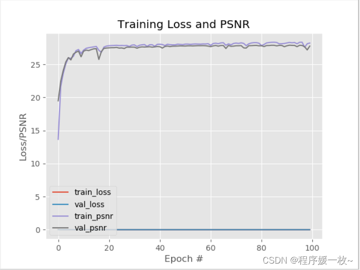
训练模型耗时3h多，结果如下：
最终验证损失为0.0019，验证PSNR得分为28.2448。

E:\python\python.exe C:\Users\admin\.IntelliJIdea2018.3\config\plugins\python\helpers\pydev\pydevd.py --multiproc --qt-support=auto --client 127.0.0.1 --port 51849 --file D:/deepLearning/py-demo/p220522/train.py
pydev debugger: process 7440 is connecting

Connected to pydev debugger (build 183.4588.61)
[INFO] loading images from disk...
2022-05-22 12:04:03.599901: I tensorflow/core/platform/cpu_feature_guard.cc:142] Your CPU supports instructions that this TensorFlow binary was not compiled to use: AVX2
[INFO] preparing data loaders...
[INFO] initializing and training model...
Epoch 1/100
...
...
...
25/25 [==============================] - 88s 4s/step - loss: 0.0020 - psnr: 28.1353 - val_loss: 0.0023 - val_psnr: 27.2020
Epoch 100/100

 1/25 [>.............................] - ETA: 1:15 - loss: 0.0015 - psnr: 29.6192
 2/25 [=>............................] - ETA: 1:12 - loss: 0.0017 - psnr: 28.7771
 3/25 [==>...........................] - ETA: 1:11 - loss: 0.0017 - psnr: 28.8514
 4/25 [===>..........................] - ETA: 1:08 - loss: 0.0017 - psnr: 28.8678
 5/25 [=====>........................] - ETA: 1:05 - loss: 0.0021 - psnr: 28.0601
 6/25 [======>.......................] - ETA: 1:01 - loss: 0.0020 - psnr: 28.0730
 7/25 [=======>......................] - ETA: 58s - loss: 0.0020 - psnr: 28.0669 
 8/25 [========>.....................] - ETA: 55s - loss: 0.0020 - psnr: 28.1785
 9/25 [=========>....................] - ETA: 52s - loss: 0.0020 - psnr: 28.0880
10/25 [===========>..................] - ETA: 49s - loss: 0.0019 - psnr: 28.3325
11/25 [============>.................] - ETA: 45s - loss: 0.0019 - psnr: 28.2930
12/25 [=============>................] - ETA: 42s - loss: 0.0019 - psnr: 28.2417
13/25 [==============>...............] - ETA: 39s - loss: 0.0019 - psnr: 28.2730
14/25 [===============>..............] - ETA: 35s - loss: 0.0019 - psnr: 28.3979
15/25 [=================>............] - ETA: 32s - loss: 0.0020 - psnr: 28.2489
16/25 [==================>...........] - ETA: 29s - loss: 0.0019 - psnr: 28.3183
17/25 [===================>..........] - ETA: 26s - loss: 0.0019 - psnr: 28.3801
18/25 [====================>.........] - ETA: 23s - loss: 0.0019 - psnr: 28.2734
19/25 [=====================>........] - ETA: 19s - loss: 0.0019 - psnr: 28.4116
20/25 [=======================>......] - ETA: 16s - loss: 0.0020 - psnr: 28.3088
21/25 [========================>.....] - ETA: 13s - loss: 0.0019 - psnr: 28.3143
22/25 [=========================>....] - ETA: 9s - loss: 0.0019 - psnr: 28.3368 
23/25 [==========================>...] - ETA: 6s - loss: 0.0019 - psnr: 28.3044
24/25 [===========================>..] - ETA: 3s - loss: 0.0019 - psnr: 28.3232
2022-05-22 14:58:37.135772: W tensorflow/core/common_runtime/base_collective_executor.cc:216] BaseCollectiveExecutor::StartAbort Out of range: End of sequence
	 [[{
    
    {
    
    node IteratorGetNext}}]]

25/25 [==============================] - 93s 4s/step - loss: 0.0019 - psnr: 28.2448 - val_loss: 0.0021 - val_psnr: 27.7841
[INFO] serializing model...

下图显示了训练历史曲线及不同时期的训练损失和PSNR分数。
在这里插入图片描述
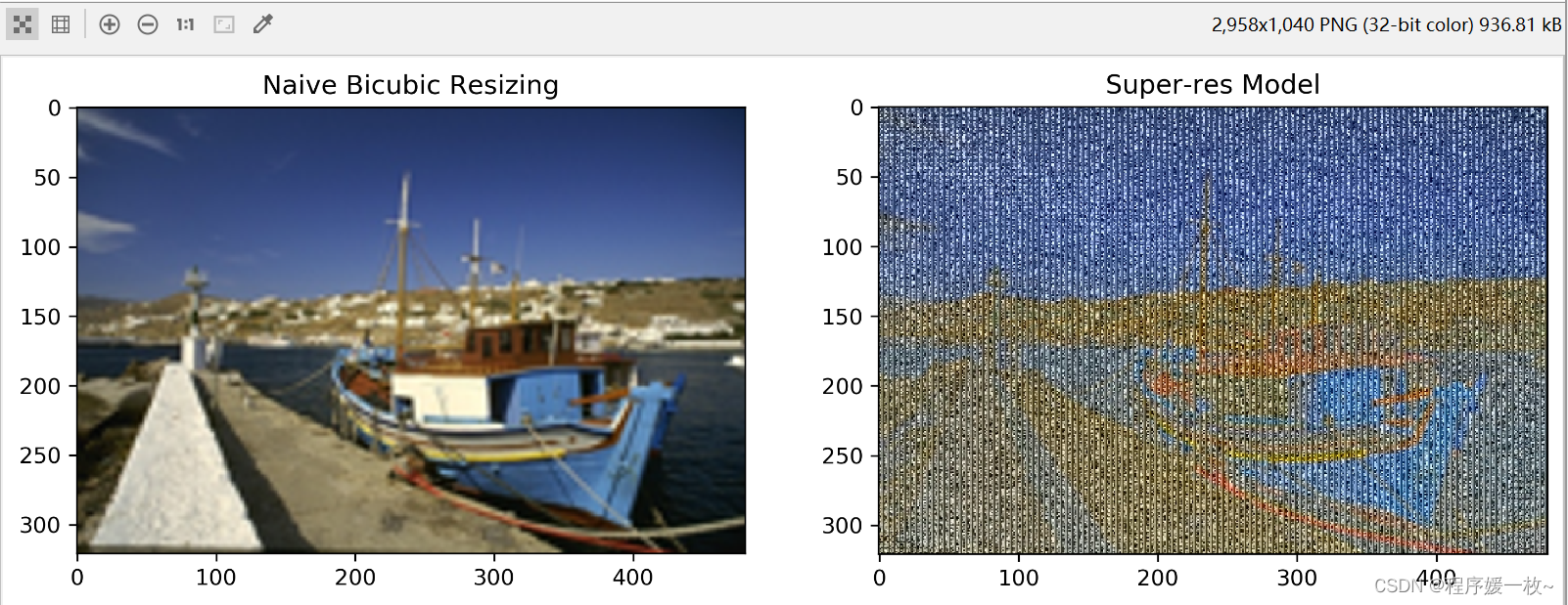
标准插值 VS RDB超分辨率模型输出效果图1如下：

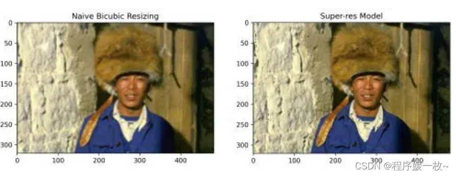
使用RDB对PSNR统计数据没有任何显著影响。然而在图像可视化后，可以看到它们在视觉质量上比单纯的双三次方法优越得多。

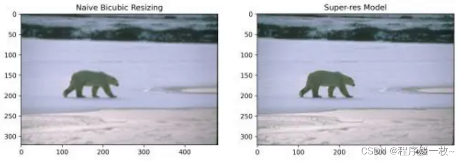
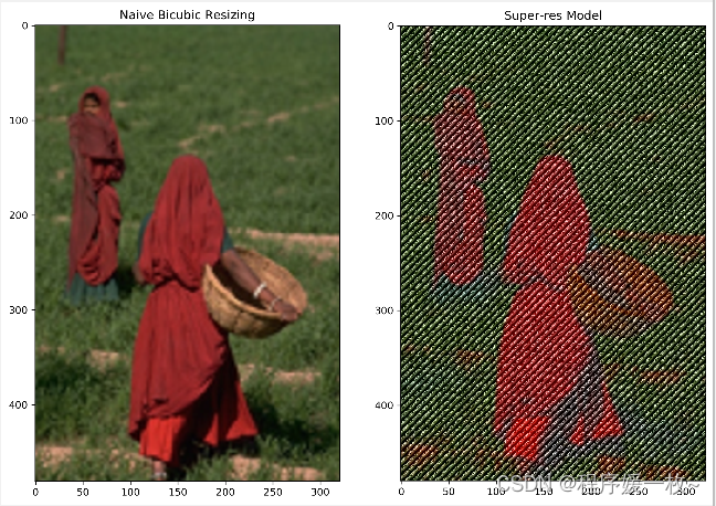
标准插值 VS RDB超分辨率模型输出效果图2如下：
在这里插入图片描述
标准插值 VS RDB超分辨率模型输出效果图3如下：
本地训练的模型不知道哪里出了问题，效果图不好；

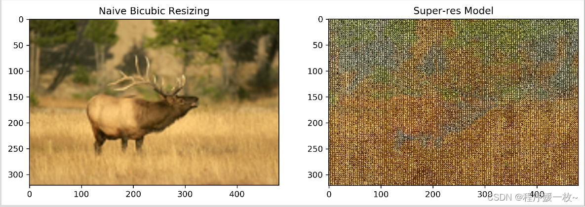
标准插值 VS RDB超分辨率模型输出效果图4如下：

标准插值 VS RDB超分辨率模型输出效果图4如下：

在这里插入图片描述

RDN能够很好地学习层次结构特征，使图像能够以非常值得称赞的视觉质量进行放大。

2. 原理

2.1 环境配置

pip install tensorflow
pip install pillow
pip install imutils

2.2 步骤

本博客将涵盖：

利用BSDS500数据集
了解残差密集块体系结构（Residual Dense Block architecture）
实现像素洗牌
展示了一系列预处理和后处理方法
训练自己的超分辨率模型
从模型结果中预测
根据标准指标评估结果
在模型上测试自己的图像

2.3 什么是像素无序超分辨率

超分辨率是一类技术的总称，其中添加了精确或接近精确的像素信息，以从低分辨率形式构建高分辨率图像，同时保持其原始质量。

像素无序超分辨率是一种上采样技术，其中图像超分辨率是通过一种相当巧妙的方法实现的。特征图是在LR（低分辨率）空间中提取的（与早期在HR（高分辨率）空间中提取的技术相反）。

该方法的亮点是一种新型高效的亚像素卷积层，它学习一组滤波器，将最终的LR特征映射放大到HR输出中。
降低了时间复杂度，因为一大块计算是在图像处于低分辨率状态时完成的。
使用了残差密集块（RDB Residual Dense Blocks），这是一种在计算当前层的输出的同时，重点关注保持前几层中提取的信息的活性的体系结构。

当从最初的层遍历到后来的层时，CNN的层将简单的特征提取到越来越复杂/抽象/高级的特征。RDB打算通过使用卷积层的密集连接网络提取尽可能多的层次特征，尽可能多地利用这一思想。

如下图所示，在RDB中所有层都是相互连接的，以确保充分提取局部特征。每个图层从所有以前的图层获得额外的输入（通过串联），并将其自己的要素贴图传递给后续图层。RDB利用了ResNets 和 Dense Blocks这俩个概念；
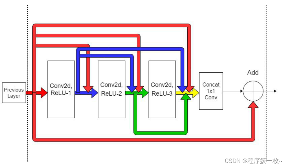在这里插入图片描述这样网络的前馈特性也得以保留。前几层的输出直接链接到当前RDB中的所有本地连接。简单来说是，来自前一层的信息将始终与当前状态一起可用，这使模型能够自适应地从各种特征中选择和优先排序。

3. 核心源码

——全部代码见

# 使用经过训练的带有RDB（Redisual Dense Blocks）亚像素CNN模型并生成超分辨率图像。它还包含几个用于图像预处理和后处理的函数。
# 模型的图表和分数表明，使用RDB不会显著提高PSNR统计数据。神奇之处在哪儿呢？测试感受一下

# output/super_res_model 存放训练好的模型
# output/training.png 样本模型评估图
# out/visualizations 存放生成的所有超分辨率图

# USAGE
# python generate_super_res.py

import os

# 导入必要的包
import cv2
import matplotlib.pyplot as plt
import numpy as np
import tensorflow as tf
from PIL import Image
from imutils import paths
from tensorflow.keras.models import load_model
from tensorflow.keras.preprocessing.image import load_img

from pyimageserach import config


# 导入必要的包


# 定义另一个函数psnr，它计算预测输出和原始图像的psnr。
# 峰值信噪比越高表示结果越好。
def psnr(orig, pred):
    # 转换目标图像为int
    orig = orig * 255.0
    orig = tf.cast(orig, tf.int32)
    orig = tf.clip_by_value(orig, 0, 255)

    # 转换预测图像为int
    pred = pred * 255.0
    pred = tf.cast(pred, tf.int32)
    pred = tf.clip_by_value(pred, 0, 255)

    # 返回psnr
    return tf.image.psnr(orig, pred, max_val=255)


def load_image(imagePath):
    print(imagePath)
    # 加载图像，使用标准三插值方法进行下采样
    orig = load_img(imagePath)
    downsampled = orig.resize((orig.size[0] // config.DOWN_FACTOR,
                               orig.size[1] // config.DOWN_FACTOR), Image.BICUBIC)

    # 返回tuple包含原始图像和下采样图像
    return (orig, downsampled)


def get_y_channel(image):
    # 将RGB图像转换为YCbCr颜色空间，并拆分为单独的通道
    ycbcr = image.convert("YCbCr")
    (y, cb, cr) = ycbcr.split()

    # 转换Y通道为numpy数组，转换为像素值为[0.0,1.0]范围
    y = np.array(y)
    y = y.astype("float32") / 255.0

    # 返回单独通道值的元组
    return (y, cb, cr)


# 根据给定的范围剪裁图像的值。
# 此函数是后处理步骤的一部分，将范围从[0.0，1.0]放大到[0，255]，并剪裁超出给定边界的任何值
def clip_numpy(image):
    # 转换图像为int值，剪切像素为[0, 255]
    image = tf.cast(image * 255.0, tf.int32)
    image = tf.clip_by_value(image, 0, 255).numpy()

    # 返回图像
    return image


def postprocess_image(y, cb, cr):
    # 进行一些初始预处理，重塑形状以匹配原始形状大小，然后将其转换为PIL图像
    y = clip_numpy(y).squeeze()
    y = y.reshape(y.shape[0], y.shape[1])
    y = Image.fromarray(y, mode="L")

    # 调整其他渠道以匹配原始图像大小
    outputCB = cb.resize(y.size, Image.BICUBIC)
    outputCR = cr.resize(y.size, Image.BICUBIC)

    # 合并调整后的通道，并以numpy数组返回
    final = Image.merge("YCbCr", (y, outputCB, outputCR)).convert("RGB")
    return np.array(final)


# 从磁盘加载测试图像路径，随机选择10个图像
print("[INFO] loading test images...")
testPaths = list(paths.list_images(config.TEST_SET))
currentTestPaths = np.random.choice(testPaths, 10)

# 从磁盘加载超分辨率模型
print("[INFO] loading model...", config.SUPER_RES_MODEL)
# superResModel = load_model(config.SUPER_RES_MODEL)
# .h5模型设置 custom_objects就可以解决，.pb不行，得先设置compile=False，然后手动compile
superResModel = load_model(config.SUPER_RES_MODEL,
                           custom_objects={
    
    "psnr": psnr})
# superResModel = load_model(config.SUPER_RES_MODEL, compile=False)
# superResModel.compile(optimizer="adam", loss="mse", metrics=[psnr])

# 遍历测试图像路径
print("[INFO] performing predictions...")
for (i, path) in enumerate(currentTestPaths):
    # 从当前路径获取原始和下采样图像路径
    (orig, downsampled) = load_image(path)

    # 提取当前图像的所有通道，进行预测
    (y, cb, cr) = get_y_channel(downsampled)
    print(y.shape, type(y))
    # y = y[None, ...]
    # print(y.shape)
    y = np.reshape(y, (y.shape[0], y.shape[1], 1))
    print('new: ', y.shape)
    upscaledY = superResModel.predict(y[None, ...])[0]

    cv2.imshow("res", upscaledY)
    # cv2.waitKey(0)

    print('res:', upscaledY.shape)
    # upscaledY = np.reshape(upscaledY, (upscaledY.shape[0], upscaledY.shape[1]))
    # print(upscaledY.shape)
    # upscaledY = upscaledY.astype(np.float32)
    # upscaledY = tf.image.convert_image_dtype(upscaledY, tf.float32)
    # upscaledY = np.array(upscaledY, np.float32)
    print(upscaledY.shape, upscaledY.dtype)

    # 对输出进行后处理，并使用标准三插值采样图像以进行比较
    finalOutput = postprocess_image(upscaledY, cb, cr)

    naiveResizing = downsampled.resize(orig.size, Image.BICUBIC)

    # 可视化结果，并存储到磁盘
    path = os.path.join(config.VISUALIZATION_PATH, f"{
      
      i}_viz.png")
    (fig, (ax1, ax2)) = plt.subplots(ncols=2, figsize=(12, 12))
    ax1.imshow(naiveResizing)
    ax2.imshow(finalOutput.astype("int"))
    ax1.set_title("Naive Bicubic Resizing")
    ax2.set_title("Super-res Model")
    fig.savefig(path, dpi=300, bbox_inches="tight")

参考

https://pyimagesearch.com/2021/09/27/pixel-shuffle-super-resolution-with-tensorflow-keras-and-deep-learning/