机器学习笔记 - 基于tensorflow从头开始构建图神经网络

1、图神经网络

        图神经网络是机器学习和深度学习领域最新兴的技术之一。在许多研究工作中，我们可以看到这些网络在结果和速度方面的成功。图神经网络成功的主要原因之一是它们使用图数据进行建模，图数据可以由数据集实体之间的结构关系组成。

        可以对图数据进行操作的神经网络可以被视为图神经网络。使用图形数据，任何神经网络都需要使用数据的顶点或节点来执行任务。假设我们正在使用任何 GNN 执行任何分类任务，那么网络需要对图数据的顶点或节点进行分类。在图数据中，节点应该带有它们的标签，以便每个节点都可以根据神经网络通过它们的标签进行分类。

        由于在大多数数据集中我们发现数据实体之间的结构关系，我们可以使用图神经网络代替其他 ML 算法，并可以利用在建模中使用图数据的好处。

        下面我们将尝试从头开始构建和实现图神经网络来构建和执行建模。我们将使用 Keras 和 TensorFlow 库实现卷积图神经网络。在这个实现中，我们将尝试将图神经网络用于节点预测任务。

2、下载数据集

        使用图神经网络需要图数据。我们这里使用的是Cora数据集。该数据集包括 2708 篇科学论文，这些论文已经分为 7 个类别，有 5429 个链接。让我们开始通过下载数据集来实现图神经网络建模。

        我们使用如下代码下载数据集

import os
from tensorflow import keras
zip_file = keras.utils.get_file(
    fname="cora.tgz",
    origin="https://linqs-data.soe.ucsc.edu/public/lbc/cora.tgz",
    extract=True,
)
data_dir = os.path.join(os.path.dirname(zip_file), "cora")

        数据集包含两个文件 

        1、cora.cites：包括引文记录

        2、cora.content：包括论文内容记录

3、读取数据并查看

import pandas as pd
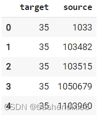
citations_data = pd.read_csv(
    os.path.join(data_dir, "cora.cites"),
    sep="\t",
    header=None,
    names=["target", "source"],
)

citations_data.head()
citations_data.describe()

         查看数据如下

         

4、数据转换并标签化

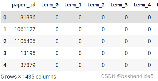
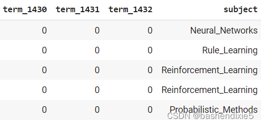
column_names = ["paper_id"] + [f"term_{idx}" for idx in range(1433)] + ["subject"]
papers_data = pd.read_csv(
    os.path.join(data_dir, "cora.content"), sep="\t", header=None, names=column_names,
)
print("Papers shape:", papers_data.shape)

papers_data.head()

class_values = sorted(papers_data["subject"].unique())
class_idc = {name: id for id, name in enumerate(class_values)}
paper_idc = {name: idx for idx, name in enumerate(sorted(papers_data["paper_id"].unique()))}

papers_data["paper_id"] = papers_data["paper_id"].apply(lambda name: paper_idc[name])
citations_data["source"] = citations_data["source"].apply(lambda name: paper_idc[name])
citations_data["target"] = citations_data["target"].apply(lambda name: paper_idc[name])
papers_data["subject"] = papers_data["subject"].apply(lambda value: class_idc[value])

        在输出中，我们可以看到该数据中有 2708 行和 1435 列的主题名称。 

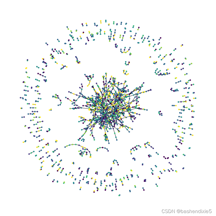
5、可视化数据

import networkx as nx
import matplotlib.pyplot as plt
plt.figure(figsize=(10, 10))
colors = papers_data["subject"].tolist()
cora_graph = nx.from_pandas_edgelist(citations_data.sample(n=1500))
subjects = list(papers_data[papers_data["paper_id"].isin(list(cora_graph.nodes))]["subject"])
nx.draw_spring(cora_graph, node_size=15, node_color=subjects)

        在输出中，我们可以看到节点是图形的表示，节点的颜色代表数据中的不同主题。正如我们所讨论的，图神经网络处理图数据，我们需要将这些数据帧转换为图数据。  

 6、制作图数据

        一个基本的图形数据可以由以下元素组成：

        节点特征：该元素表示数组中的节点数和特征数。我们在本文中使用的数据集具有可用作节点的论文信息，node_features 是每篇论文的单词存在二进制向量。

        边：这是节点之间链接的稀疏矩阵，表示两个维度中的边数。在我们的数据集中，链接是论文引用。

        边权重：这是一个可选元素，是一个数组。该数组下的值表示边数，这是节点之间的量化。

import tensorflow as tf
feature_names = set(papers_data.columns) - {"paper_id", "subject"}
# Create an edges array (sparse adjacency matrix) of shape [2, num_edges].
edges = citations_data[["source", "target"]].to_numpy().T
# Create an edge weights array of ones.
edge_weights = tf.ones(shape=edges.shape[1])
# Create a node features array of shape [num_nodes, num_features].
node_features = tf.cast(
    papers_data.sort_values("paper_id")[feature_names].to_numpy(), dtype=tf.dtypes.float32
)
# Create graph info tuple with node_features, edges, and edge_weights.
graph_info = (node_features, edges, edge_weights)

print("Edges shape:", edges.shape)
print("Nodes shape:", node_features.shape)

7、实现图神经网络

        需要制作一个可以处理图形数据的层。

from tensorflow.keras import layers
class GraphConvLayer(layers.Layer):
    def __init__(
        self,
        hidden_units,
        dropout_rate=0.2,
        aggregation_type="mean",
        combination_type="concat",
        normalize=False,
        *args,
        **kwargs,
    ):
        super(GraphConvLayer, self).__init__(*args, **kwargs)

        self.aggregation_type = aggregation_type
        self.combination_type = combination_type
        self.normalize = normalize

        self.ffn_prepare = create_ffn(hidden_units, dropout_rate)
        if self.combination_type == "gated":
            self.update_fn = layers.GRU(
                units=hidden_units,
                activation="tanh",
                recurrent_activation="sigmoid",
                dropout=dropout_rate,
                return_state=True,
                recurrent_dropout=dropout_rate,
            )
        else:
            self.update_fn = create_ffn(hidden_units, dropout_rate)

    def prepare(self, node_repesentations, weights=None):
        # node_repesentations shape is [num_edges, embedding_dim].
        messages = self.ffn_prepare(node_repesentations)
        if weights is not None:
            messages = messages * tf.expand_dims(weights, -1)
        return messages

    def aggregate(self, node_indices, neighbour_messages):
        # node_indices shape is [num_edges].
        # neighbour_messages shape: [num_edges, representation_dim].
        num_nodes = tf.math.reduce_max(node_indices) + 1
        if self.aggregation_type == "sum":
            aggregated_message = tf.math.unsorted_segment_sum(
                neighbour_messages, node_indices, num_segments=num_nodes
            )
        elif self.aggregation_type == "mean":
            aggregated_message = tf.math.unsorted_segment_mean(
                neighbour_messages, node_indices, num_segments=num_nodes
            )
        elif self.aggregation_type == "max":
            aggregated_message = tf.math.unsorted_segment_max(
                neighbour_messages, node_indices, num_segments=num_nodes
            )
        else:
            raise ValueError(f"Invalid aggregation type: {self.aggregation_type}.")

        return aggregated_message

    def update(self, node_repesentations, aggregated_messages):
        # node_repesentations shape is [num_nodes, representation_dim].
        # aggregated_messages shape is [num_nodes, representation_dim].
        if self.combination_type == "gru":
            # Create a sequence of two elements for the GRU layer.
            h = tf.stack([node_repesentations, aggregated_messages], axis=1)
        elif self.combination_type == "concat":
            # Concatenate the node_repesentations and aggregated_messages.
            h = tf.concat([node_repesentations, aggregated_messages], axis=1)
        elif self.combination_type == "add":
            # Add node_repesentations and aggregated_messages.
            h = node_repesentations + aggregated_messages
        else:
            raise ValueError(f"Invalid combination type: {self.combination_type}.")

        # Apply the processing function.
        node_embeddings = self.update_fn(h)
        if self.combination_type == "gru":
            node_embeddings = tf.unstack(node_embeddings, axis=1)[-1]

        if self.normalize:
            node_embeddings = tf.nn.l2_normalize(node_embeddings, axis=-1)
        return node_embeddings

    def call(self, inputs):
        """Process the inputs to produce the node_embeddings.

        inputs: a tuple of three elements: node_repesentations, edges, edge_weights.
        Returns: node_embeddings of shape [num_nodes, representation_dim].
        """

        node_repesentations, edges, edge_weights = inputs
        # Get node_indices (source) and neighbour_indices (target) from edges.
        node_indices, neighbour_indices = edges[0], edges[1]
        # neighbour_repesentations shape is [num_edges, representation_dim].
        neighbour_repesentations = tf.gather(node_repesentations, neighbour_indices)

        # Prepare the messages of the neighbours.
        neighbour_messages = self.prepare(neighbour_repesentations, edge_weights)
        # Aggregate the neighbour messages.
        aggregated_messages = self.aggregate(node_indices, neighbour_messages)
        # Update the node embedding with the neighbour messages.
        return self.update(node_repesentations, aggregated_messages)

8、实现节点分类器

class GNNNodeClassifier(tf.keras.Model):
    def __init__(
        self,
        graph_info,
        num_classes,
        hidden_units,
        aggregation_type="sum",
        combination_type="concat",
        dropout_rate=0.2,
        normalize=True,
        *args,
        **kwargs,
    ):
        super(GNNNodeClassifier, self).__init__(*args, **kwargs)

        # Unpack graph_info to three elements: node_features, edges, and edge_weight.
        node_features, edges, edge_weights = graph_info
        self.node_features = node_features
        self.edges = edges
        self.edge_weights = edge_weights
        # Set edge_weights to ones if not provided.
        if self.edge_weights is None:
            self.edge_weights = tf.ones(shape=edges.shape[1])
        # Scale edge_weights to sum to 1.
        self.edge_weights = self.edge_weights / tf.math.reduce_sum(self.edge_weights)

        # Create a process layer.
        self.preprocess = create_ffn(hidden_units, dropout_rate, name="preprocess")
        # Create the first GraphConv layer.
        self.conv1 = GraphConvLayer(
            hidden_units,
            dropout_rate,
            aggregation_type,
            combination_type,
            normalize,
            name="graph_conv1",
        )
        # Create the second GraphConv layer.
        self.conv2 = GraphConvLayer(
            hidden_units,
            dropout_rate,
            aggregation_type,
            combination_type,
            normalize,
            name="graph_conv2",
        )
        # Create a postprocess layer.
        self.postprocess = create_ffn(hidden_units, dropout_rate, name="postprocess")
        # Create a compute logits layer.
        self.compute_logits = layers.Dense(units=num_classes, name="logits")

    def call(self, input_node_indices):
        # Preprocess the node_features to produce node representations.
        x = self.preprocess(self.node_features)
        # Apply the first graph conv layer.
        x1 = self.conv1((x, self.edges, self.edge_weights))
        # Skip connection.
        x = x1 + x
        # Apply the second graph conv layer.
        x2 = self.conv2((x, self.edges, self.edge_weights))
        # Skip connection.
        x = x2 + x
        # Postprocess node embedding.
        x = self.postprocess(x)
        # Fetch node embeddings for the input node_indices.
        node_embeddings = tf.gather(x, input_node_indices)
        # Compute logits
        return self.compute_logits(node_embeddings)

9、训练并测试

import numpy as np
train, test = [], []

for _, group in papers_data.groupby("subject"):
    # Select around 50% of the dataset for training.
    random_selection = np.random.rand(len(group.index)) <= 0.5
    train.append(group[random_selection])
    test.append(group[~random_selection])

train = pd.concat(train).sample(frac=1)
test = pd.concat(test).sample(frac=1)

print("Train data shape:", train.shape)
print("Test data shape:", test.shape)

num_features = len(feature_names)
num_classes = len(class_idc)
hidden_units = [32, 32]
learning_rate = 0.01
dropout_rate = 0.5
num_epochs = 300
batch_size = 256

def create_ffn(hidden_units, dropout_rate, name=None):
    fnn_layers = []

    for units in hidden_units:
        fnn_layers.append(layers.BatchNormalization())
        fnn_layers.append(layers.Dropout(dropout_rate))
        fnn_layers.append(layers.Dense(units, activation=tf.nn.gelu))

    return keras.Sequential(fnn_layers, name=name)

gnn_model = GNNNodeClassifier(
    graph_info=graph_info,
    num_classes=num_classes,
    hidden_units=hidden_units,
    dropout_rate=dropout_rate,
    name="gnn_model",
)

print("GNN output shape:", gnn_model([1, 10, 100]))

gnn_model.summary()


x_train = train[feature_names].to_numpy()
x_test = test[feature_names].to_numpy()
# Create train and test targets as a numpy array.
y_train = train["subject"]
y_test = test["subject"]



x_train = train.paper_id.to_numpy()
def run_experiment(model, x_train, y_train):
    # Compile the model.
    model.compile(
        optimizer=keras.optimizers.Adam(learning_rate),
        loss=keras.losses.SparseCategoricalCrossentropy(from_logits=True),
        metrics=[keras.metrics.SparseCategoricalAccuracy(name="acc")],
    )
    # Create an early stopping callback.
    early_stopping = keras.callbacks.EarlyStopping(
        monitor="val_acc", patience=50, restore_best_weights=True
    )
    # Fit the model.
    history = model.fit(
        x=x_train,
        y=y_train,
        epochs=num_epochs,
        batch_size=batch_size,
        validation_split=0.15,
        callbacks=[early_stopping],
    )

    return history
history = run_experiment(gnn_model, x_train, y_train)

fig, ax1 = plt.subplots(1, figsize=(15, 5))

ax1.plot(history.history["loss"])
ax1.plot(history.history["val_loss"])
ax1.legend(["train", "test"], loc="upper right")
ax1.set_xlabel("Epochs")
ax1.set_ylabel("Loss")


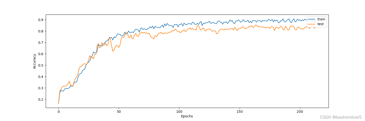
fig, ax2 = plt.subplots(1, figsize=(15, 5))
ax2.plot(history.history["acc"])
ax2.plot(history.history["val_acc"])
ax2.legend(["train", "test"], loc="upper right")
ax2.set_xlabel("Epochs")
ax2.set_ylabel("Accuracy")
plt.show()

        损失曲线如下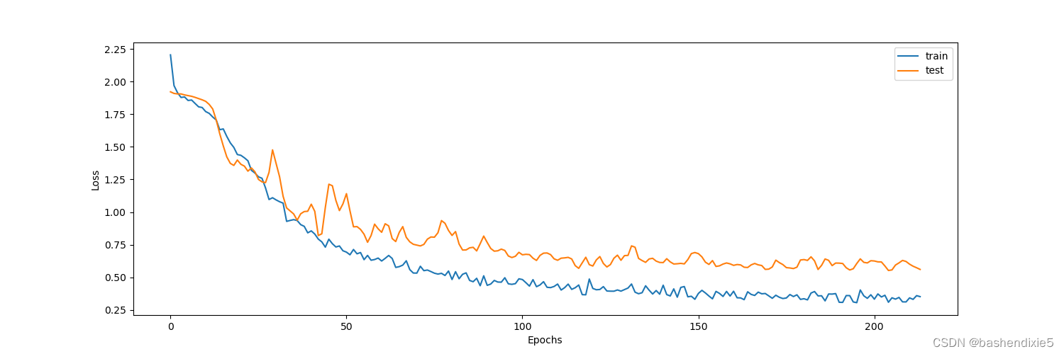

         准确率曲线如下