大家好,研究了两天终于把 YOLOV4 预测阶段的完整代码复现出来了。本文只用函数方法,最直观的向大家展示代码。强烈建议大家在阅读本文之前,先看以下文章:
(1)YOLOV4特征提取网络:https://blog.csdn.net/dgvv4/article/details/123818580
(2)先验框解码调整:https://blog.csdn.net/dgvv4/article/details/124076352
(3)NMS非极大值抑制:https://blog.csdn.net/dgvv4/article/details/124062839
由于本文篇幅有点长,可以用右侧的目录栏跳转。理论部分我已经在上面几篇博文中写的很清楚了,这里就不再赘述了。
完整代码在我的Gitee中,有需要的自取:
https://gitee.com/dgvv4/yolo-target-detection/tree/master/YOLOV4%E9%A2%84%E6%B5%8B%E4%BB%A3%E7%A0%81
YOLOV4的VOC数据集的权重文件下载地址:
链接:https://pan.baidu.com/s/1WEq4eZ6UFsByWGZQf0AE1w 提取码:snlw
先放张图看效果:


1. 特征提取网络
这个部分在之前的文章中已经构建过,理论方面不懂的可以看上面的链接。这里就简单提一下。
1.1 骨干特征提取网络
CSPDarkNet53 骨干特征提取网络在 YOLOV3 的 DarkNet53网络 的基础上引入了 CSP结构。该结构增强了卷积神经网络的学习能力;移除了计算瓶颈;降低了显存的使用;加快了网络的推理速度。
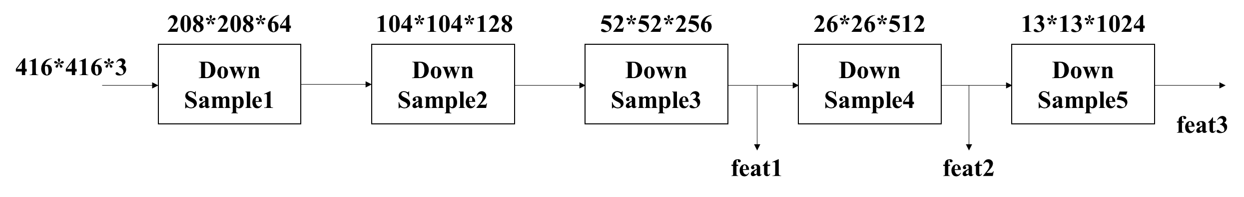
输入图像的shape为[416,416,3],网络不断进行下采样来获得更高的语义信息,输出三个有效特征层,feat1的shape为 [52,52,256] ,feat2的shape为[26,26,512] ,feat3的shape为[13,13,1024]
代码如下,文件命名为 CSPDarknet53.py
import tensorflow as tf
from tensorflow import keras
from tensorflow.keras import layers, regularizers

#(1)Mish激活函数
def mish(x):
    # x*tanh(ln(1+ex))
    x = x * tf.math.tanh(tf.math.softplus(x))
    return x

#(2)标准卷积块
def conv_block(inputs, filters, kernel_size, strides):
    # 卷积+BN+Mish
    x = layers.Conv2D(filters, kernel_size, strides,
                      padding='same', use_bias=False,  # 有BN不要偏置
                      kernel_regularizer=regularizers.l2(5e-4))(inputs)  # l2正则化

    x = layers.BatchNormalization()(x)
    x = mish(x)

    return x

#(3)残差块
def res_block(inputs, filters, num):

    residual = inputs  # 残差边
    # 1*1卷积调整通道
    x = conv_block(inputs, filters//2, kernel_size=(1,1), strides=1)
    # 3*3卷积提取特征
    x = conv_block(x, filters//2 if num!=1 else filters, kernel_size=(3,3), strides=1)
    # 残差连接输入和输出
    x = layers.Add()([x, residual])

    return x

#(4)CSP结构
def csp_bolck(inputs, filters, num):

    # 卷积下采样
    x = conv_block(inputs, filters, kernel_size=(3,3), strides=2)

    # num!=1时1*1卷积在通道维度上会下降一半
    shortcut = conv_block(x, filters//2 if num!=1 else filters, (1,1), strides=1)  # 残差边
    mainconv = conv_block(x, filters//2 if num!=1 else filters, (1,1), strides=1)  # 主干卷积

    # 重复执行残差结构
    for _ in range(num):
        mainconv = res_block(inputs=mainconv, filters=filters, num=num)

    # 1*1卷积调整通道
    mainconv = conv_block(mainconv, filters//2 if num!=1 else filters, (1,1), strides=1)

    # 输入和输出在通道维度堆叠
    x = layers.concatenate([mainconv, shortcut])

    # 1*1卷积整合通道
    x = conv_block(x, filters, (1,1), strides=1)

    return x

#(5)主干网络
def cspdarknet(inputs):

    # [416,416,3]==>[416,416,32]
    x = conv_block(inputs, filters=32, kernel_size=(3,3), strides=1)
    # [416,416,32]==>[208,208,64]
    x = csp_bolck(x, filters=64, num=1)
    # [208,208,64]==>[104,104,128]
    x = csp_bolck(x, filters=128, num=2)

    # [104,104,128]==>[52,52,256]
    x = csp_bolck(x, filters=256, num=8)
    feat1 = x

    # [52,52,256]==>[26,26,512]
    x = csp_bolck(x, filters=512, num=8)
    feat2 = x

    # [26,26,512]==>[13,13,1024]
    x = csp_bolck(x, filters=1024, num=4)
    feat3 = x

    return feat1, feat2, feat3
1.2 SPP结构
对网络模型输出的 feat3 先经过三个卷积层调整通道数,然后分别使用池化核size为 5*5,9*9,13*13 的最大池化,通过padding='same' 使得池化前后的特征图的shape是完全相同的。然后将原始输入和三种池化的结果特征图在通道维度上堆叠。最后经过三次卷积融合通道信息。

代码如下,文件命名为 SPP.py
import tensorflow as tf
from tensorflow import keras
from tensorflow.keras import layers
from CSPDarknet53 import cspdarknet  # 导入网络模型
from CSPDarknet53 import conv_block  # 导入标准卷积块

def spp(inputs):

    # 获取网络的三个输出特征层
    feat1, feat2, feat3 = cspdarknet(inputs)

    # 对最后一个输出特征层进行3次卷积
    # [13,13,1024]==>[13,13,512]
    p5 = conv_block(feat3, filters=512, kernel_size=(1,1), strides=1)
    # [13,13,512]==>[13,13,1024]
    p5 = conv_block(p5, filters=1024, kernel_size=(3,3), strides=1)
    # [13,13,1024]==>[13,13,512]
    p5 = conv_block(p5, filters=512, kernel_size=(1,1), strides=1)

    # 经过不同尺度的最大池化后相堆叠
    maxpool1 = layers.MaxPooling2D(pool_size=(13,13), strides=1, padding='same')(p5)
    maxpool2 = layers.MaxPooling2D(pool_size=(9,9), strides=1, padding='same')(p5)
    maxpool3 = layers.MaxPooling2D(pool_size=(5,5), strides=1, padding='same')(p5)

    # 四种尺度在通道维度上堆叠[13,13,2048]
    p5 = layers.concatenate([maxpool1, maxpool2, maxpool3, p5])

    # 三次卷积调整通道数
    # [13,13,2048]==>[13,13,512]
    p5 = conv_block(p5, filters=512, kernel_size=(1,1), strides=1)
    # [13,13,512]==>[13,13,1024]
    p5 = conv_block(p5, filters=1024, kernel_size=(3,3), strides=1)
    # [13,13,1024]==>[13,13,512]
    p5 = conv_block(p5, filters=512, kernel_size=(1,1), strides=1)

    return feat1, feat2, p5
1.3 PANet 金字塔
PANet 将网络输出的有效特征层和SPP结构的输出进行特征融合,它是由两个特征金字塔组成,一个是将低层的语义信息向高层融合,另一个是将高层的语义信息向低层融合。

代码如下,文件命名为 PANet.py
import tensorflow as tf
from tensorflow import keras
from tensorflow.keras import layers
from CSPDarknet53 import conv_block  # 网络模型和标准卷积块
from SPP import spp  # 导入spp加强特征提取模块

# 5次卷积操作提取特征减少参数量
def five_conv(x, filters):
    x = conv_block(x, filters, (1,1), strides=1)
    x = conv_block(x, filters*2, (3,3), strides=1)
    x = conv_block(x, filters, (1,1), strides=1)
    x = conv_block(x, filters*2, (3,3), strides=1)
    x = conv_block(x, filters, (1,1), strides=1)
    return x

def panet(inputs):

    # 获得网络的三个有效输出特征层
    feat1, feat2, p5 = spp(inputs)

    #(1)
    # 对spp结构的输出进行卷积和上采样
    # [13,13,512]==>[13,13,256]==>[26,26,256]
    p5_upsample = conv_block(p5, filters=256, kernel_size=(1,1), strides=1)
    p5_upsample = layers.UpSampling2D(size=(2,2))(p5_upsample)

    # 对feat2特征层卷积后再与p5_upsample堆叠
    # [26,26,512]==>[26,26,256]==>[26,26,512]
    p4 = conv_block(feat2, filters=256, kernel_size=(1,1), strides=1)
    p4 = layers.concatenate([p4, p5_upsample])

    # 堆叠后进行5次卷积[26,26,512]==>[26,26,256]
    p4 = five_conv(p4, filters=256)

    #(2)
    # 对p4卷积上采样
    # [26,26,256]==>[26,26,512]==>[52,52,512]
    p4_upsample = conv_block(p4, filters=128, kernel_size=(1,1), strides=1)
    p4_upsample = layers.UpSampling2D(size=(2,2))(p4_upsample)

    # feat1层卷积后与p4_upsample堆叠
    # [52,52,256]==>[52,52,128]==>[52,52,256]
    p3 = conv_block(feat1, filters=128, kernel_size=(1,1), strides=1)
    p3 = layers.concatenate([p3, p4_upsample])

    # 堆叠后进行5次卷积[52,52,256]==>[52,52,128]
    p3 = five_conv(p3, filters=128)

    # 存放第一个特征层的输出
    p3_output = p3

    #(3)
    # p3卷积下采样和p4堆叠
    # [52,52,128]==>[26,26,256]==>[26,26,512]
    p3_downsample = conv_block(p3, filters=256, kernel_size=(3,3), strides=2)
    p4 = layers.concatenate([p3_downsample, p4])

    # 堆叠后的结果进行5次卷积[26,26,512]==>[26,26,256]
    p4 = five_conv(p4, filters=256)

    # 存放第二个有效特征层的输出
    p4_output = p4

    #(4)
    # p4卷积下采样和p5堆叠
    # [26,26,256]==>[13,13,512]==>[13,13,1024]
    p4_downsample = conv_block(p4, filters=512, kernel_size=(3,3), strides=2)
    p5 = layers.concatenate([p4_downsample, p5])

    # 堆叠后进行5次卷积[13,13,1024]==>[13,13,512]
    p5 = five_conv(p5, filters=512)

    # 存放第三个有效特征层的输出
    p5_output = p5

    # 返回输出层结果
    return p3_output, p4_output, p5_output
1.4 YOLO预测头
YOLOHead 由一个3*3卷积层和一个1*1卷积层构成,3*3卷积整合之前获得的所有特征信息,1*1卷积获得三个有效特征层的输出结果。
代码如下,命名为 YOLOHEAD.py
import tensorflow as tf
from tensorflow import keras
from tensorflow.keras import layers, Model
from PANet import panet  # 导入panet加强特征提取方法
from CSPDarknet53 import conv_block  # 导入标准卷积快

# 对PANet的特征输出层处理获得最终的预测结果
def yoloHead(inputs, num_anchors, num_classes):
    '''
    num_anchors每个网格包含先验框的数量, num_classes分类数
    num_anchors(5+num_classes)代表: 每个先验框有5+num_classes个参数, 即(x,y,w,h,c)和20个类别的条件概率
    每一个特征层的输出代表: 每一个网格上每一个先验框内部是否包含物体, 以及包含物体的种类, 和先验框的调整参数
    '''

    # 获得三个有效特征层
    p3_output, p4_output, p5_output = panet(inputs)

    # 3*3卷积[52,52,128]==>[52,52,256]
    p3_output = conv_block(p3_output, filters=256, kernel_size=(3,3), strides=1)
    # [52,52,256]==>[52,52,num_anchors(5+num_classes)]
    p3_output = conv_block(p3_output, filters=num_anchors*(5+num_classes),
                           kernel_size=(1,1), strides=1)

    # [26,26,256]==>[26,26,516]
    p4_output = conv_block(p4_output, filters=512, kernel_size=(3,3), strides=1)
    # [26,26,512]==>[26,26,num_anchors(5+num_classes)]
    p4_output = conv_block(p4_output, filters=num_anchors*(5+num_classes),
                           kernel_size=(1,1), strides=1)

    # [13,13,512]==>[13,13,1024]
    p5_output = conv_block(p5_output, filters=1024, kernel_size=(3,3), strides=1)
    # [13,13,1024]==>[13,13,num_anchors(5+num_classes)]
    p5_output = conv_block(p5_output, filters=num_anchors*(5+num_classes),
                           kernel_size=(1,1), strides=1)

    # 返回三个有效特征层
    return p5_output, p4_output, p3_output
1.5 模型构建
输入是416*416的图像,输出是三个有效特征层,13*13检测层负责预测大目标,26*26检测层负责预测中目标,52*52的特征层负责预测小目标。
代码如下,文件命名为 model.py
import tensorflow as tf
from tensorflow import keras
from YOLOHEAD import yoloHead  # 加载网络的预测头

# 构造模型
def MODEL(inputs, num_anchors, num_classes, summary=False):

    # 接收输出的三个有效特征层
    p5_output, p4_output, p3_output = yoloHead(inputs, num_anchors, num_classes)
    # 构造模型
    model = keras.Model(inputs, [p5_output, p4_output, p3_output])
    # 是否查看模型结构
    if summary:
        model.summary()
    # 返回模型
    return model
2. 先验框解码,获得预测框
首先要对网络的输出特征层解码,它们的shape分别是 [52, 52, (3*(5+num_classes))],[26, 26, (3*(5+num_classes))],[13, 13, (3*(5+num_classes))]。
其中通道数 3*(5+num_classes) 可以理解为:每个网格生成 3 个预测框,每个预测框包含了预测框相较于先验框的偏移量,坐标偏移量(tx, ty),宽高偏移量(tw, th),预测框中是否包含目标物体 c,预测框内的物体属于每个类别的条件概率num_classes,在VOC数据集中num_classes=20。其中 (tx, ty) 是负无穷到正无穷的任何数,(tw, th) 是归一化后的宽高。

以某个网格的先验框的调整为例,如下图所示,虚线框代表:和物体的真实标签框 iou 值最大的那个先验框,该先验框的宽高为(pw, ph);蓝色框代表微调先验框后生成的预测框。
(cx,cy)是先验框中心点所在的网格的左上坐标(归一化后的坐标),由于坐标偏移量 (tx,ty) 可以是从负无穷到正无穷的任何数,为了防止坐标调整偏移过大,给偏移量添加sigmoid函数。将坐标偏移量限制在0-1之间,将预测框的中心点限制在它所在的网格内。

接下来将预测框的坐标和高度宽度归一化处理,再将归一化后的预测框信息映射到原始图像的大小,例如,在 13*13 的图像上得到的归一化后的预测框,需要映射到 1280*720 的原始图片大小上
代码如下,命名为 anchors.py
# 先验框解码调整预测框
import tensorflow as tf

#(一)对某一个输出特征层解码
def anchors_decode(feats, anchors, num_classes, inputs_shape):
    '''
    feats是某一个特征层的输出结果, 如shape=[b, 13, 13, 3*(5+num_classes)]
    anchors代表每个特征层, 每个网格会生成三个先验框[3,2]
    num_classes代表分类类别的数量
    inputs_shape代表输入图像的高宽[416,416]
    '''
    # 计算每个网格先验框的个数=3
    num_anchors = len(anchors)
    # 获得网格的高宽(h,w)=(13,13)
    grid_shape = feats.shape[1:3]

    #(1)构造网格,将图像划分成13*13个网格
    # 获得网格的x坐标 (13)==>[1,13,1,1]
    grid_x = tf.reshape(range(grid_shape[1]), shape=[1,-1,1,1])
    # 在y和anchors维度上复制扩张[1,13,1,1]==>[13,13,3,1]
    grid_x = tf.tile(grid_x, multiples=[grid_shape[0], 1, num_anchors, 1])

    # 同理获得网格的y坐标(13)==>[13,1,1,1]==>[13,13,3,1]
    grid_y = tf.tile(tf.reshape(range(grid_shape[0]), shape=[-1,1,1,1]), multiples=[1, grid_shape[1], num_anchors, 1])

    # 在通道维度上合并[13,13,3,2], 并且转换成tf.float32类型
    grid = tf.cast(tf.concat([grid_x, grid_y], axis=-1), dtype=tf.float32)

    #(2)调整先验框宽高shape, 13*13个网格,每个网格3个先验框,每个先验框(x,y)
    # [3,2]==>[1,1,3,2]
    anchors_tensor = tf.reshape(anchors, shape=[1,1,num_anchors,2])
    # 扩充[1,1,3,2]==>[13,13,3,2]
    anchors_tensor = tf.tile(anchors_tensor, multiples=[grid_shape[0], grid_shape[1], 1, 1])
    # 转换数据类型
    anchors_tensor = tf.cast(anchors_tensor, dtype=tf.float32)

    #(3)调整网络输出层的shape
    # [b,13,13,num_anchors*(5+num_classes)]==>[b,13,13,num_anchors,5+num_classes]
    feats = tf.reshape(feats, [-1, grid_shape[0], grid_shape[1], num_anchors, 5+num_classes])
    '''
    代表13*13个网格, 每个网格有3个先验框, 每个先验框有(5+num_classes)项信息
    其中, 5代表: 中心点坐标(x,y), 宽高(w,h), 置信度c
    num_classes: 检测框属于某个类别的条件概率, VOC数据集中等于20
    '''

    #(4)调整网格的先验框中心坐标和宽高
    # 归一化中心点坐标偏移量,把预测框中心点限制在该网格中
    anchors_xy = tf.nn.sigmoid(feats[..., :2])
    box_xy = anchors_xy + grid
    # 坐标归一化
    grid_shape_wh = tf.cast(grid_shape[::-1], feats.dtype)  #
    box_xy = box_xy / grid_shape_wh

    # 调整先验框宽高,得到预测框
    anchors_wh = tf.exp(feats[..., 2:4])
    box_wh = anchors_wh * anchors_tensor
    # 宽高度归一化
    inputs_shape_wh = tf.cast(inputs_shape[::-1], feats.dtype)
    box_wh = box_wh / inputs_shape_wh

    # 获得预测框的置信度和每个类别的条件概率
    box_conf = tf.nn.sigmoid(feats[..., 4:5])
    box_prob = tf.nn.sigmoid(feats[..., 5:])

    # 返回预测框的信息
    return box_xy, box_wh, box_conf, box_prob


#(二)将归一化后的预测框信息转换为对应的原图坐标
def correct_box(box_xy, box_wh, inputs_shape, image_shape):
    # 调整shape, y轴放前面方便宽高相乘
    box_yx = box_xy[..., ::-1]
    box_hw = box_wh[..., ::-1]

    # 调整输入图像的数据类型
    inputs_shape = tf.cast(inputs_shape, box_yx.dtype)
    image_shape = tf.cast(image_shape, box_hw.dtype)

    # 计算预测框在网格上的左上角和右下角坐标
    box_min = box_yx - (box_hw / 2.0)
    box_max = box_yx + (box_hw / 2.0)

    # 保存网格的左上和右下坐标
    boxes  = tf.concat([box_min[..., 0:1], box_min[..., 1:2], box_max[..., 0:1], box_max[..., 1:2]], axis=-1)
    # 获得原图上的左上和右下坐标
    boxes = boxes * tf.concat([image_shape, image_shape], axis=-1)

    return boxes


#(三)计算一个特征层的检测框坐标和类别的概率
def anchors_prediction(feats, anchors, num_classes, inputs_shape, image_shape):
    '''
    feats是某一个特征层的输出结果, 如shape=[b, 13, 13, 3*(5+num_classes)]
    anchors代表每个特征层, 每个网格会生成三个先验框[3,2]
    num_classes代表分类类别的数量
    image_shape:原始图像大小
    inputs_shape:网络输入的图片大小(h,w)=416*416
    '''
    # 获得某个特征层输出的预测框信息
    box_xy, box_wh, box_conf, box_prob = anchors_decode(feats, anchors, num_classes, inputs_shape)

    # 获得在原图像上的预测框
    boxes = correct_box(box_xy, box_wh, inputs_shape, image_shape)
    # [4]==>[n,4]
    boxes = tf.reshape(boxes, shape=[-1, 4])

    # 获得每个类别的真实概率
    box_scores = box_conf * box_prob
    # [num_classes]==>[n,num_classes]
    box_scores = tf.reshape(box_scores, shape=[-1,num_classes])

    # 返回每个框的坐标和每个类别的概率
    return boxes, box_scores
3. NMS非极大值抑制剔除冗余框
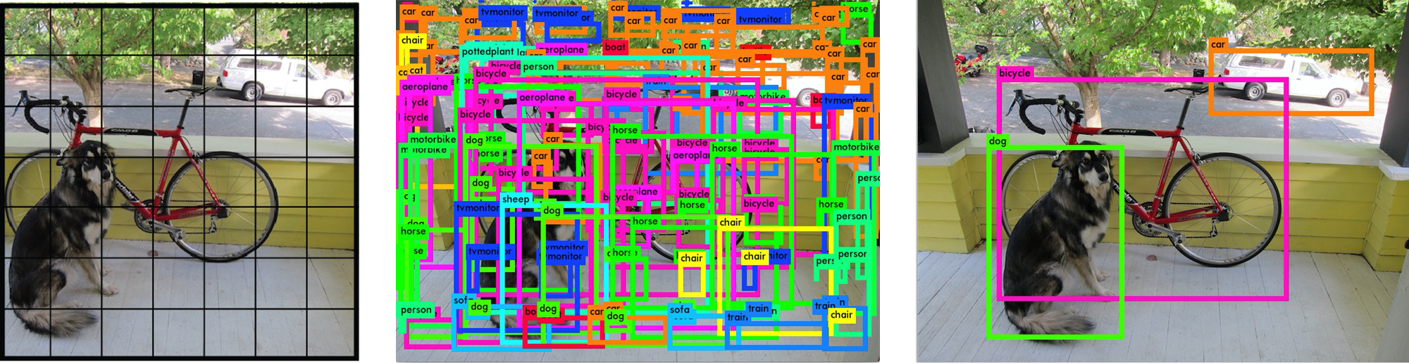
图像经过神经网络模型运算,会得到多个目标预测框。然而,每个目标只有一个真实标签框,算法却会生成多个预测框,这样会造成检测框冗余或预测错误的情况。因此,深度神经网络通过非极大值抑制 NMS 来筛选预测框,去掉交并比更大并且置信度较低的冗余检测框,剩下置信度较高,定位较准确的预测框。
代码如下,命名为 NMS.py
import tensorflow as tf
import numpy as np
from anchors import anchors_prediction  # 导入对网络每一输出层的解码方法

# 对所有输出层解码,并使用非极大值抑制
def predict(feats, image_shape, num_classes, pre_anchors, conf_thresh, nms_thresh, max_boxes=20):
    '''
    feats:代表模型的三个有效输出特征层
    image_shape:原始图像的(h,w)
    max_boxes:最大预测框数量
    conf_thresh:分类概率小于这个值的框被删除
    nms_thresh:两个框计算交并比, iou小于这个值被保留, 删除重复的框
    '''
    # 每个特征层对应的三个先验框
    anchor_mask = [[6,7,8], [3,4,5], [0,1,2]]

    boxes = []  # 存放每张图的预测框坐标
    box_scores = []  # 每个预测框的类别概率

    # 获得网络输入的图像的shape=416*416
    inputs_shape = tf.constant([416,416])

    # 获取三个有效输出特征层的预测框坐标和类别概率
    for i in range(len(feats)):
        #获取每个输出层的预测框坐标和概率
        feat_boxes, feat_box_scores = anchors_prediction(feats=feats[i],
                                                         anchors=pre_anchors[anchor_mask[i]],  # 每个输出层对应的3个先验框
                                                         num_classes=num_classes,  # 分类数
                                                         inputs_shape=inputs_shape,  # 网络的输出图像大小[416,416]
                                                         image_shape=image_shape)  # 原始图像大小
        # 保存每一层的预测框坐标和概率
        # feat_boxes.shape=[2028,4], feat_box_scores.shape=[2028,20]
        boxes.append(feat_boxes)
        box_scores.append(feat_box_scores)

    # 调整排序方式,放在一行中 [[], [], []]==>[ , , ]
    boxes = tf.concat(boxes, axis=0)
    box_scores = tf.concat(box_scores, axis=0)

    # 设置一个阈值,保留概率高于该阈值的预测框
    # mask.shape=[3*2028, 20]
    mask = (box_scores) > conf_thresh
    # 设置每张图片最多出现几个预测框
    max_boxes = tf.constant(max_boxes, tf.int32)

    '''
    box_score是每个检测框对应的20个类别的概率
    mask是每个检测框的20个类别的概率是否满足要求
    '''

    # 保存每个预测框的坐标, 概率, 类别名称
    predict_boxes = []
    predict_score = []
    predict_classes = []

    # 对每一个类别删除重复的框
    for c in range(num_classes):
        # 取出所有类为c且满足最小概率要求的box
        class_boxes = tf.boolean_mask(boxes, mask[:, c])
        # 取出所有类为c的分数
        class_box_scores = tf.boolean_mask(box_scores[:, c], mask[:, c])
        # 非极大抑制
        nms_index = tf.image.non_max_suppression(class_boxes, class_box_scores, max_boxes, iou_threshold = nms_thresh)

        # 取出筛选后的结果
        class_boxes = tf.gather(class_boxes, nms_index)  # 检测框坐标
        class_box_scores = tf.gather(class_box_scores, nms_index)  # 每个框的类别概率
        classes = tf.ones_like(class_box_scores, dtype=tf.int32) * c  # 1*c获得类别索引

        # 保存筛选后的预测框坐标、概率、类别
        predict_boxes.append(class_boxes)
        predict_score.append(class_box_scores)
        predict_classes.append(classes)

    # 重新排序预测框, 放在同一行
    predict_boxes = tf.concat(predict_boxes, axis=0)
    predict_score = tf.concat(predict_score, axis=0)
    predict_classes = tf.concat(predict_classes, axis=0)

    return predict_boxes, predict_score, predict_classes
4. 视频目标检测
首先对读入的帧图像预处理,opencv读入的图片是BGR类型,需要转换成RGB,然后再转换成 Image 类型,调整图像尺寸从1280*720调整为416*416,然后再将像素值归一化,并为单张图像扩充batchsize维度 [h, w, c] ==> [b, h, w, c]。将预处理后的图像传入网络预测 yolo_model.predict(img)。
这里使用的 VOC数据集的权重和分类,以及聚类后的先验框的宽高比
代码如下,命名为 results.py
import cv2
import numpy as np
from PIL import Image
import tensorflow as tf
from tensorflow import keras
from model import MODEL  # 导入网络模型结构
from NMS import predict  # 导入预测框处理方法
# 调用GPU加速
gpus = tf.config.experimental.list_physical_devices(device_type='GPU')
for gpu in gpus:
    tf.config.experimental.set_memory_growth(gpu, True)

# -------------------------------------------- #
# yolov4权重文件路径, 视频文件路径
# -------------------------------------------- #
yolo_weights = 'yolo4_voc_weights.h5'
video_path = 'D:/deeplearning/video/car.mp4'
cap = cv2.VideoCapture(video_path)  # 视频捕获

# -------------------------------------------- #
# class_names: VOC数据集的分类名
# anchors: 先验框的长宽
# num_anchors: 每个网格生成几个先验框
# num_classes: 一共有几个类别
# inputs_shape: 输入图像的尺寸
# inputs: 网络输入层
# conf_thresh:分类概率小于这个值的框被删除
# nms_thresh:两个框计算交并比, iou小于这个值被保留, 删除重复的框
# -------------------------------------------- #
class_names = ['aeroplane', 'bicycle', 'bird', 'boat', 'bottle', 'bus', 'car', 'cat', 'chair', 'cow',
              'diningtable', 'dog', 'horse', 'motorbike', 'person', 'pottedplant', 'sheep', 'sofa', 'train', 'tvmonitor']

anchors = np.array([[12, 16],  [19, 36],  [40, 28],  [36, 75],  [76, 55],  [72, 146],  [142, 110],  [192, 243],  [459, 401]])
num_anchors = 3
num_classes = len(class_names)
input_shape = [416,416,3]
inputs = keras.Input(shape=input_shape)
conf_thresh = 0.6
nms_thresh = 0.4

# ----------------------------------------------------- #
# 模型构造, 加载权重, 自定义的网络层名报错就用by_name=True
# ----------------------------------------------------- #
yolo_model = MODEL(inputs, num_anchors, num_classes, summary=False)
yolo_model.load_weights(yolo_weights, by_name=True)

# ----------------------------------------------------- #
# 图像预处理
# ----------------------------------------------------- #
def preprocessing(image, inputs_shape):

    # opencv读入的图像是BGR格式,转换成RGB
    image = cv2.cvtColor(image, cv2.COLOR_BGR2RGB)
    # 转换成Image类型
    image = Image.fromarray(np.uint8(image))
    # 调整图像尺寸
    image_data = image.resize(size=(inputs_shape[1], inputs_shape[0]))
    # 改变数据类型
    image_data = np.array(image_data, dtype=np.float32)
    # 归一化
    image_data = image_data / 255.0
    # 添加batch维度 [416,416,3]==>[1,416,416,3]
    image_data = np.expand_dims(image_data, axis=0)

    return image_data

# ----------------------------------------------------- #
# 处理视频帧图像
# ----------------------------------------------------- #
while True:
    # 返回图像是否读取成功success,以及读取的帧图像img
    success, img = cap.read()
    # 将读入的图像复制一份
    frame = img.copy()
    # 原始输入图像的(h,w)
    image_shape = img.shape[0:2]
    # 图像预处理
    img = preprocessing(img, input_shape)

    # 返回模型输出的三个有效特征层
    p5_output, p4_output, p3_output = yolo_model.predict(img)

    # 整合一下输出特征层
    feats = [p5_output, p4_output, p3_output]

    # ----------------------------------------------------- #
    # 将输出的预测框信息解码、调整先验框、非极大值抑制
    # feats:代表模型的三个有效输出特征层
    # image_shape:原始图像的(h,w)
    # num_classes:分类类别数
    # anchors:先验框的高宽
    # conf_thresh:分类概率小于这个值的框被删除
    # nms_thresh:两个框计算交并比, iou小于这个值被保留, 删除重复的框
    # max_boxes:最大预测框数量
    # ----------------------------------------------------- #
    # predict_boxes预测框左上坐标和宽高
    # predict_score预测框的类别概率
    # predict_classes预测框所属类别的索引
    # ----------------------------------------------------- #
    predict_boxes, predict_score, predict_classes = predict(feats, image_shape, num_classes, anchors, conf_thresh, nms_thresh, max_boxes=100)

    # ----------------------------------------------------- #
    # 绘制预测框
    # ----------------------------------------------------- #
    for box, score, class_index in zip(predict_boxes, predict_score, predict_classes):

        # 获取预测框的左上坐标和宽高
        box_y1, box_x1, box_y2, box_x2 = box[0], box[1], box[2], box[3]
        # 每个预测框的类别名称
        class_name = class_names[class_index]
        # 将名称和分数组合在一起, 字符串
        class_name_score = class_name + ': ' + str(round(score.numpy(),2))

        # 绘制预测框
        cv2.rectangle(frame, (box_x1, box_y1), (box_x2, box_y2), color=(0,255,0), thickness=2)
        # 显示类别和概率
        cv2.putText(frame, class_name_score, (box_x1, box_y1-5), cv2.FONT_HERSHEY_COMPLEX, 1, (0,0,255), 2)

    # ----------------------------------------------------- #
    # 显示图像
    # ----------------------------------------------------- #
    cv2.imshow('frame', frame)  # 传入窗口名和帧图像
    # 每帧图像滞留10毫秒后消失,按下键盘上的ESC键退出程序
    if cv2.waitKey(10) & 0xFF == 27:
        break

# 释放视频资源
cap.release()
cv2.destroyAllWindows()
视频效果展示:
