【yolov4】基于yolov4深度学习网络目标检测MATLAB仿真

       YOLO发展至YOLOv3时，基本上这个系列都达到了一个高潮阶段，很多实际任务中，都会见到YOLOv3的身上，而对于较为简单和场景，比如没有太密集的目标和极端小的目标，多数时候仅用YOLOv2即可。除了YOLO系列，也还有其他很多优秀的工作，比如结构同样简洁的RetinaNet和SSD。后者SSD其实也会常在实际任务中见到，只不过就性能而言，要略差于YOLOv3，当然，这也是因为SSD并没有去做后续的升级，反倒很多新工作如RFB-Net、DSSD等工作都将其作为baseline。论性能，RetinaNet当然是不输于YOLOv3的，只是，相较于YOLOv3，RetinaNet的一个较为致命的问题就是：速度太慢。而这一个问题的主要原因就是RetinaNet使用较大的输出图像尺寸和较重的检测头。

yolov4的创新点
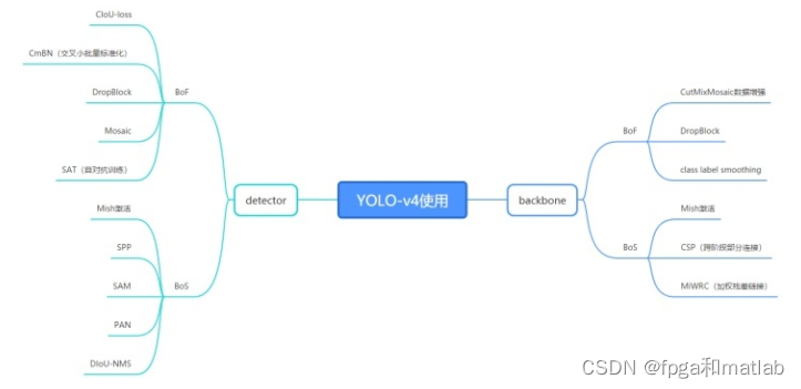
1.输入端的创新点：训练时对输入端的改进，主要包括Mosaic数据增强、cmBN、SAT自对抗训练

2.BackBone主干网络：各种方法技巧结合起来，包括：CSPDarknet53、Mish激活函数、Dropblock

3.Neck：目标检测网络在BackBone和最后的输出层之间往往会插入一些层，比如Yolov4中的SPP模块、FPN+PAN结构

4.Head：输出层的锚框机制和Yolov3相同，主要改进的是训练时的回归框位置损失函数CIOU_Loss，以及预测框筛选的nms变为DIOU_nms

       通俗的讲，就是说这个YOLO-v4算法是在原有YOLO目标检测架构的基础上，采用了近些年CNN领域中最优秀的优化策略，从数据处理、主干网络、网络训练、激活函数、损失函数等各个方面都有着不同程度的优化，虽没有理论上的创新，但是会受到许许多多的工程师的欢迎，各种优化算法的尝试。文章如同于目标检测的trick综述，效果达到了实现FPS与Precision平衡的目标检测 new baseline。

          yolov4 网络结构的采用的算法，其中保留了yolov3的head部分，修改了主干网络为CSPDarknet53，同时采用了SPP（空间金字塔池化）的思想来扩大感受野，PANet作为neck部分。

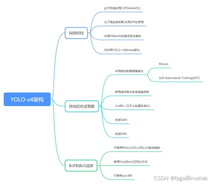
yolov4在技术处理的思维导图：

1.MATLAB源码

clc;
clear;
close all;
warning off;
addpath(genpath(pwd));

%****************************************************************************
%更多关于matlab和fpga的搜索“fpga和matlab”的CSDN博客:
%matlab/FPGA项目开发合作
%https://blog.csdn.net/ccsss22?type=blog
%****************************************************************************
%% Download Pretrained Network
% Set the modelName from the above ones to download that pretrained model.
modelName = 'YOLOv4-coco';
model = helper.downloadPretrainedYOLOv4(modelName);
net = model.net;

%% Load Data
% Unzip the vehicle images and load the vehicle ground truth data. 
unzip vehicleDatasetImages.zip
data = load('vehicleDatasetGroundTruth.mat');
vehicleDataset = data.vehicleDataset;

% Add the full path to the local vehicle data folder.
vehicleDataset.imageFilename = fullfile(pwd, vehicleDataset.imageFilename);


rng('default')
shuffledIndices = randperm(height(vehicleDataset));
idx = floor(0.6 * length(shuffledIndices));
trainingDataTbl = vehicleDataset(shuffledIndices(1:idx), :);
testDataTbl = vehicleDataset(shuffledIndices(idx+1:end), :);

% Create an image datastore for loading the images.
imdsTrain = imageDatastore(trainingDataTbl.imageFilename);
imdsTest = imageDatastore(testDataTbl.imageFilename);
 
% Create a datastore for the ground truth bounding boxes.
bldsTrain = boxLabelDatastore(trainingDataTbl(:, 2:end));
bldsTest = boxLabelDatastore(testDataTbl(:, 2:end));

% Combine the image and box label datastores.
trainingData = combine(imdsTrain, bldsTrain);
testData = combine(imdsTest, bldsTest);

helper.validateInputData(trainingData);
helper.validateInputData(testData);

%% Data Augmentation
augmentedTrainingData = transform(trainingData, @helper.augmentData);
 

augmentedData = cell(4,1);
for k = 1:4
    data = read(augmentedTrainingData);
    augmentedData{k} = insertShape(data{1,1}, 'Rectangle', data{1,2});
    reset(augmentedTrainingData);
end
figure
montage(augmentedData, 'BorderSize', 10)

%% Preprocess Training Data
% Specify the network input size. 
networkInputSize = net.Layers(1).InputSize;
 

preprocessedTrainingData = transform(augmentedTrainingData, @(data)helper.preprocessData(data, networkInputSize));
 
% Read the preprocessed training data.
data = read(preprocessedTrainingData);

% Display the image with the bounding boxes.
I = data{1,1};
bbox = data{1,2};
annotatedImage = insertShape(I, 'Rectangle', bbox);
annotatedImage = imresize(annotatedImage,2);
figure
imshow(annotatedImage)

% Reset the datastore.
reset(preprocessedTrainingData);

%% Modify Pretrained YOLO v4 Network

rng(0)
trainingDataForEstimation = transform(trainingData, @(data)helper.preprocessData(data, networkInputSize));
numAnchors = 9;
[anchorBoxes, meanIoU] = estimateAnchorBoxes(trainingDataForEstimation, numAnchors);

% Specify the classNames to be used in the training.
classNames = {'vehicle'};


[lgraph, networkOutputs, anchorBoxes, anchorBoxMasks] = configureYOLOv4(net, classNames, anchorBoxes, modelName);

%% Specify Training Options
numEpochs = 90;
miniBatchSize = 4;
learningRate = 0.001;
warmupPeriod = 1000;
l2Regularization = 0.001;
penaltyThreshold = 0.5;
velocity = [];

%% Train Model
if canUseParallelPool
   dispatchInBackground = true;
else
   dispatchInBackground = false;
end

mbqTrain = minibatchqueue(preprocessedTrainingData, 2,...
        "MiniBatchSize", miniBatchSize,...
        "MiniBatchFcn", @(images, boxes, labels) helper.createBatchData(images, boxes, labels, classNames), ...
        "MiniBatchFormat", ["SSCB", ""],...
        "DispatchInBackground", dispatchInBackground,...
        "OutputCast", ["", "double"]);



% Convert layer graph to dlnetwork.
net = dlnetwork(lgraph);

% Create subplots for the learning rate and mini-batch loss.
fig = figure;
[lossPlotter, learningRatePlotter] = helper.configureTrainingProgressPlotter(fig);

iteration = 0;
% Custom training loop.
for epoch = 1:numEpochs
      
    reset(mbqTrain);
    shuffle(mbqTrain);
    
    while(hasdata(mbqTrain))
        iteration = iteration + 1;
       
        [XTrain, YTrain] = next(mbqTrain);
        
        % Evaluate the model gradients and loss using dlfeval and the
        % modelGradients function.
        [gradients, state, lossInfo] = dlfeval(@modelGradients, net, XTrain, YTrain, anchorBoxes, anchorBoxMasks, penaltyThreshold, networkOutputs);

        % Apply L2 regularization.
        gradients = dlupdate(@(g,w) g + l2Regularization*w, gradients, net.Learnables);

        % Determine the current learning rate value.
        currentLR = helper.piecewiseLearningRateWithWarmup(iteration, epoch, learningRate, warmupPeriod, numEpochs);
        
        % Update the network learnable parameters using the SGDM optimizer.
        [net, velocity] = sgdmupdate(net, gradients, velocity, currentLR);

        % Update the state parameters of dlnetwork.
        net.State = state;
        
        % Display progress.
        if mod(iteration,10)==1
            helper.displayLossInfo(epoch, iteration, currentLR, lossInfo);
        end
            
        % Update training plot with new points.
        helper.updatePlots(lossPlotter, learningRatePlotter, iteration, currentLR, lossInfo.totalLoss);
    end
end

% Save the trained model with the anchors.
anchors.anchorBoxes = anchorBoxes;
anchors.anchorBoxMasks = anchorBoxMasks;

save('yolov4_trained', 'net', 'anchors');

%% Evaluate Model
confidenceThreshold = 0.5;
overlapThreshold = 0.5;

% Create a table to hold the bounding boxes, scores, and labels returned by
% the detector. 
numImages = size(testDataTbl, 1);
results = table('Size', [0 3], ...
    'VariableTypes', {'cell','cell','cell'}, ...
    'VariableNames', {'Boxes','Scores','Labels'});

% Run detector on images in the test set and collect results.
reset(testData)
while hasdata(testData)
    % Read the datastore and get the image.
    data = read(testData);
    image = data{1};
    
    % Run the detector.
    executionEnvironment = 'auto';
    [bboxes, scores, labels] = detectYOLOv4(net, image, anchors, classNames, executionEnvironment);
    
    % Collect the results.
    tbl = table({bboxes}, {scores}, {labels}, 'VariableNames', {'Boxes','Scores','Labels'});
    results = [results; tbl];
end

% Evaluate the object detector using Average Precision metric.
[ap, recall, precision] = evaluateDetectionPrecision(results, testData);

% The precision-recall (PR) curve shows how precise a detector is at varying 
% levels of recall. Ideally, the precision is 1 at all recall levels.

% Plot precision-recall curve.
figure
plot(recall, precision)
xlabel('Recall')
ylabel('Precision')
grid on
title(sprintf('Average Precision = %.2f', ap))

%% Detect Objects Using Trained YOLO v4
reset(testData)
data = read(testData);

% Get the image.
I = data{1};

% Run the detector.
executionEnvironment = 'auto';
[bboxes, scores, labels] = detectYOLOv4(net, I, anchors, classNames, executionEnvironment);

% Display the detections on image.
if ~isempty(scores)
    I = insertObjectAnnotation(I, 'rectangle', bboxes, scores);
end
figure
imshow(I)

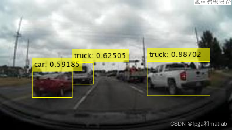
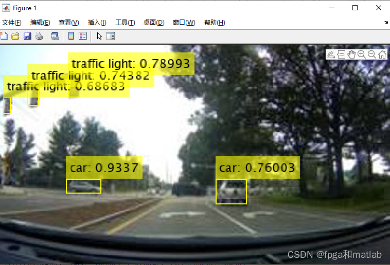
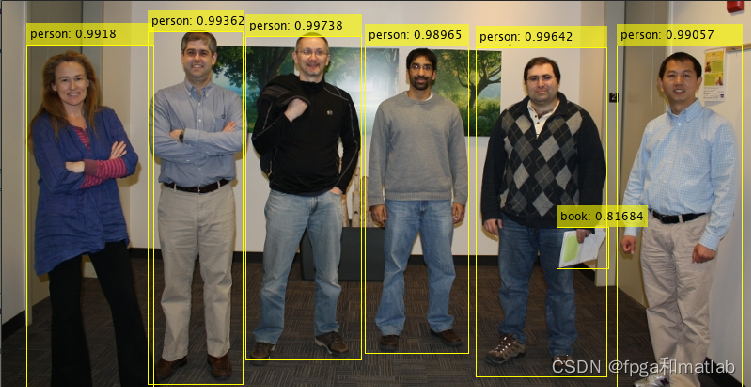
2.yolov4仿真效果

 

 

 

资源