TensorFlow深度学习框架学习（二）：TensorFlow实现线性支持向量机（SVM）

SVM的原理可以参考李航的《统计学习方法》
具体代码如下，代码都有注释的

#1、导入必要的库
import matplotlib.pyplot as plt
import numpy as np
import tensorflow as tf
from sklearn import datasets

#2、创建一个计算图会话，加载需要的数据集。
sess = tf.Session()
iris = datasets.load_iris()
#在iris中的data这个字段里面，取第一列（其为花萼长度）和第四列（为花萼宽度）的特征变量
x_vals = np.array([[x[0], x[3]] for x in iris.data])
#iris中的target字段里面有3个数值：0,1,2；其中将0（山鸢尾花）都设置为1，其他都设置为-1
y_vals = np.array([1 if y==0 else -1 for y in iris.target])

#3、将数据集分割为：训练集和测试集;
#训练集的x和y分别为x_vals_train 和 y_vals_train
#测试集的x和y分别为x_vals_test 和 y_vals_test
train_indices = np.random.choice(len(x_vals), round(len(x_vals)*0.8), replace=False)
test_indices = np.array(list(set(range(len(x_vals))) - set(train_indices)))
x_vals_train = x_vals[train_indices]
x_vals_test = x_vals[test_indices]
y_vals_train = y_vals[train_indices]
y_vals_test = y_vals[test_indices]

#4、设置批量大小，占位符，模型变量
batch_size = 100

x_data = tf.placeholder(shape=[None, 2], dtype=tf.float32)
y_target = tf.placeholder(shape=[None, 1], dtype=tf.float32)

#这里的A，其实就是ω
A = tf.Variable(tf.random_normal(shape=[2,1]))
b = tf.Variable(tf.random_normal(shape=[1,1]))

#5、声明模型输出
model_output = tf.subtract(tf.matmul(x_data, A), b)

#6、声明最大间隔损失函数，这里的损失函数是特定的一个损失函数，详见《TensorFlow机器学习指南》68页
#定义一个函数来计算向量的L2范数。
l2_norm = tf.reduce_sum(tf.square(A))

#增加间隔参数α= 0.1
alpha = tf.constant([0.01])

classification_term = tf.reduce_mean(tf.maximum(0., tf.subtract(1., tf.multiply(model_output, y_target))))

loss = tf.add(classification_term, tf.multiply(alpha, l2_norm))

#7、声明预测函数和准确度函数，用来评估训练集和测试集训练的准确度：
prediction = tf.sign(model_output)
accuracy = tf.reduce_mean(tf.cast(tf.equal(prediction, y_target), tf.float32))

#8、声明优化器函数
my_opt = tf.train.GradientDescentOptimizer(0.01)
train_step = my_opt.minimize(loss)
#初始化模型代码
init = tf.global_variables_initializer()
sess.run(init)

#9、遍历迭代训练模型，记录训练集和测试集训练的损失和准确度
loss_vec = []
train_accuracy = []
test_accuracy = []
for i in range(1000):
    rand_index = np.random.choice(len(x_vals_train), size=batch_size)
    rand_x = x_vals_train[rand_index]
    rand_y = np.transpose([y_vals_train[rand_index]])
    sess.run(train_step, feed_dict={x_data: rand_x, y_target: rand_y})

    temp_loss = sess.run(loss, feed_dict={x_data: rand_x, y_target: rand_y})
    loss_vec.append(temp_loss)

    train_acc_temp = sess.run(accuracy, feed_dict={x_data: x_vals_train, y_target:np.transpose([y_vals_train])}) 
    train_accuracy.append(train_acc_temp)

    test_acc_temp = sess.run(accuracy, feed_dict={x_data: x_vals_test, y_target:np.transpose([y_vals_test])})
    test_accuracy.append(test_acc_temp)

    '''
    if(i+1)%100==0:
        print('Step #'+ str(i+1) + ' A = ' + str(sess.run(A)) + ' b = ' + str(sess.run(b)))
        print('Loss = ' + str(temp_loss))
    '''

#10、抽取数据
[[a1], [a2]] = sess.run(A)
[ [b] ] = sess.run(b)
#slope是斜率的意思，intercept是截距的意思
slope = -a2/a1
y_intercept = b/a1

#下面这句话的意思是将x_vals中的第二列单独取出赋值给x1_vals
x1_vals = [d[1] for d in x_vals]

#best_fit这个best_fit是根据x1_vals计算出超平面上的x0_vals值
#超平面是a1 * x0_vals + a2 * x1_vals - b = 0 所以 x0_vals = -a2/a1 * x1_vals + b/a1 ; 
best_fit = []
for i in x1_vals:
    best_fit.append(slope*i+y_intercept)

#setosa表示山鸢尾花，enumerate表示枚举
#为什么底下用enumerate？因为i表示的是x_vals的索引值，而使用enumerate可以直接获得x_vals的索引值
setosa_x = [d[1] for i,d in enumerate(x_vals) if y_vals[i]==1]
setosa_y = [d[0] for i,d in enumerate(x_vals) if y_vals[i]==1]
#not_setosa表示不是山鸢尾花
not_setosa_x = [d[1] for i,d in enumerate(x_vals) if y_vals[i]==-1]
not_setosa_y = [d[0] for i,d in enumerate(x_vals) if y_vals[i]==-1]

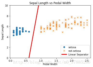
#12、使用Python代码绘制数据的线性分类器、准确度和损失图
#首先，先画出将样本分类的图
plt.plot(setosa_x, setosa_y, 'o', label='setosa')
plt.plot(not_setosa_x, not_setosa_y, 'x', label='not-setosa')
plt.plot(x1_vals, best_fit, 'r-', label='Linear Separator', linewidth=3)
plt.ylim([0, 10])
plt.legend(loc='lower right')
plt.title('Sepal Length vs Pedal Width')
plt.xlabel('Pedal Width')
plt.ylabel('Sepal Length')
plt.show()

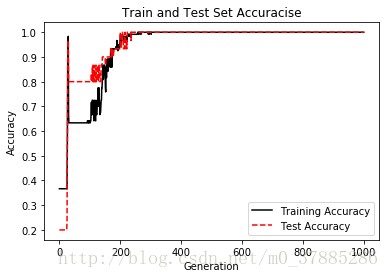
#训练集和测试集迭代的准确度
plt.plot(train_accuracy, 'k-', label='Training Accuracy')
plt.plot(test_accuracy, 'r--', label='Test Accuracy')
plt.title('Train and Test Set Accuracise')
plt.xlabel('Generation')
plt.ylabel('Accuracy')
plt.legend(loc='lower right')
plt.show()

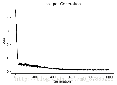
#最大间隔图
plt.plot(loss_vec, 'k-')
plt.title('Loss per Generation')
plt.xlabel('Generation')
plt.ylabel('Loss')
plt.show()

最后得到的结果如下：