支持向量机SVM----学习笔记二（代码实践一线性分类）

本篇主要记录如何使用sklearn去实现线性SVM，使用的是鸢尾花数据集，在对SVM进行分类前，和KNN一样我们首先，要对数据进行标准化处理，这是因为SVM寻找的是使margin最大的区间中间的那根线，而我们衡量margin的方式是数据点之间的距离，如果数据点在不同维度上量纲不同的话，那对于距离的估计就是有问题的。

例如在下图中，横轴范围在0-1，纵轴范围却在0-10000，对应的决策边界只能这么划分，虽然看上去尺度很短,但是纵轴是从0-10000，纵轴上很短的距离都代表一个很大的数。

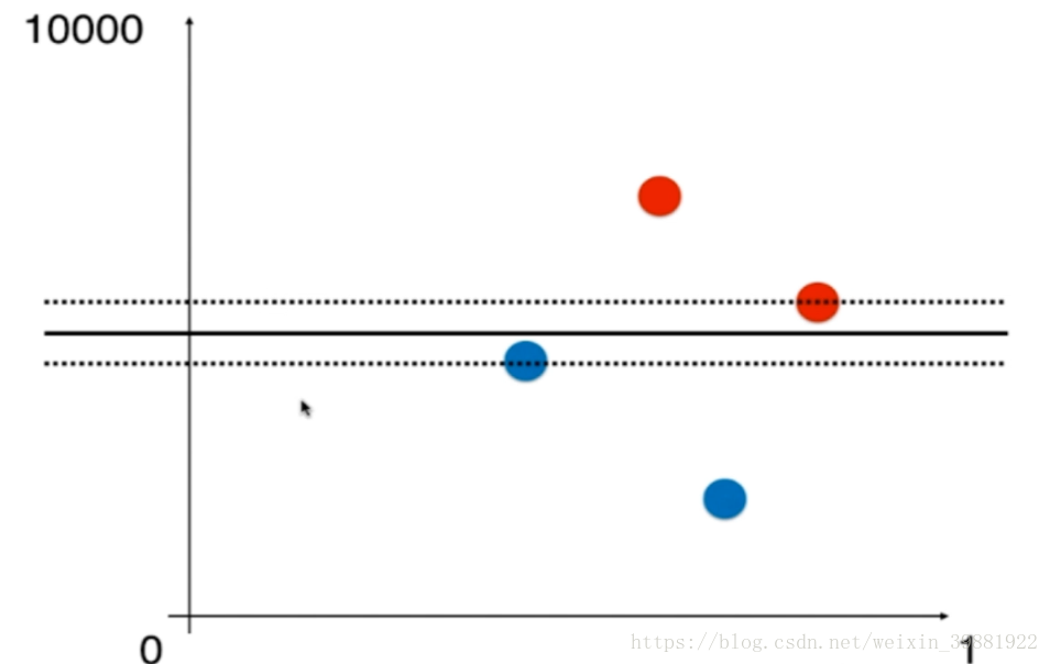
但如果横纵项范围都是在0-1范围里，此时决策边界变为如下所示：

总之，对于SVM来说，如果特征在不同的维度上数据尺度不同的话，将会非常严重影响SVM得到的决策边界，为了避免这种情况的出现，再使用SVM之前，应对数据进行标准化处理。

Scikit-learn中的SVM

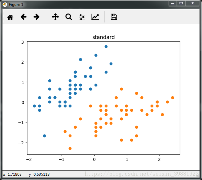
1.准备数据

import numpy as np
import matplotlib.pyplot as plt
from sklearn import datasets
iris=datasets.load_iris()

X=iris.data
print(X)
Y=iris.target
print(Y)

#处理二分类问题，所以只针对Y=0,1的行，然后从这些行中取X的前两列
x=X[Y<2,:2]
y=Y[Y<2]

#target=0的点标红，target=1的点标蓝,点的横坐标为data的第一列，点的纵坐标为data的第二列
plt.scatter(x[y==0,0],x[y==0,1],color='red')
plt.scatter(x[y==1,0],x[y==1,1],color='blue')

plt.show()

X:
 [[ 5.1  3.5  1.4  0.2]
 [ 4.9  3.   1.4  0.2]
 [ 4.7  3.2  1.3  0.2]
 [ 4.6  3.1  1.5  0.2]
 [ 5.   3.6  1.4  0.2]
 [ 5.4  3.9  1.7  0.4]
 [ 4.6  3.4  1.4  0.3]
 ...
 [ 6.5  3.   5.2  2. ]
 [ 6.2  3.4  5.4  2.3]
 [ 5.9  3.   5.1  1.8]]
Y:
 [0 0 0 0 0 0 0 0 0 0 0 0 0 0 0 0 0 0 0 0 0 0 0 0 0 0 0 0 0 0 0 0 0 0 0 0 0
 0 0 0 0 0 0 0 0 0 0 0 0 0 1 1 1 1 1 1 1 1 1 1 1 1 1 1 1 1 1 1 1 1 1 1 1 1
 1 1 1 1 1 1 1 1 1 1 1 1 1 1 1 1 1 1 1 1 1 1 1 1 1 1 2 2 2 2 2 2 2 2 2 2 2
 2 2 2 2 2 2 2 2 2 2 2 2 2 2 2 2 2 2 2 2 2 2 2 2 2 2 2 2 2 2 2 2 2 2 2 2 2
 2 2]
x:
 [[ 5.1  3.5]
 [ 4.9  3. ]
 [ 4.7  3.2]
 [ 4.6  3.1]
 [ 5.   3.6]
 [ 5.4  3.9]
 ...
 [ 6.2  2.9]
 [ 5.1  2.5]
 [ 5.7  2.8]]
y:
 [0 0 0 0 0 0 0 0 0 0 0 0 0 0 0 0 0 0 0 0 0 0 0 0 0 0 0 0 0 0 0 0 0 0 0 0 0
 0 0 0 0 0 0 0 0 0 0 0 0 0 1 1 1 1 1 1 1 1 1 1 1 1 1 1 1 1 1 1 1 1 1 1 1 1
 1 1 1 1 1 1 1 1 1 1 1 1 1 1 1 1 1 1 1 1 1 1 1 1 1 1]

2.对数据进行标准化

#在用SVM进行分类前，要对数据进行标准化
from sklearn.preprocessing import StandardScaler
#实例化一个标准化对象
standardScaler=StandardScaler()
standardScaler.fit(x)
#完成了对数据x的标准化
x_standard=standardScaler.transform(x)

3.使用SVM算法对此数据进行分类

当C很大时，趋向硬间隔

#引入线性SVM SVC:Support vector classifier
from sklearn.svm import LinearSVC
#C越大，允许的容错空间越小，越偏向与hard margin（线性可分）
svc1=LinearSVC(C=1e9)
svc1.fit(x_standard,y)
print(svc1)
def plot_decision_boundary(model,axis):
    x0,x1=np.meshgrid(
        np.linspace(axis[0],axis[1],int((axis[1]-axis[0])*100)),
        np.linspace(axis[2], axis[3], int((axis[3]-axis[2])*100))
    )
    x_new=np.c_[x0.ravel(),x1.ravel()]
    #对横坐标axis[2]到axis[3]x0，纵坐标axis[0]到axis[1]x1进行组合，组合成n行两列的数据点，对这些数据点进行预测
    y_predict=model.predict(x_new).reshape(x0.shape)

    #引入ListedColormap用于生成非渐变的颜色映射
    from matplotlib.colors import ListedColormap
    # 自定义colormap
    custom_cmap=ListedColormap(['#EF9A9A','#FFF59D','#90CAF9'])
    #contourf(x, y, z)对等高线间的填充区域进行填充（使用不同的颜色）x和y为两个等长一维数组，第三个参数z为二维数组（表示平面点xi,yi映射的函数值）。
    plt.contourf(x0,x1,y_predict,linewidth=5,cmap=custom_cmap)

plot_decision_boundary(svc1,axis=[-3,3,-3,3])
plt.scatter(x_standard[y==0,0],x_standard[y==0,1])
plt.scatter(x_standard[y==1,0],x_standard[y==1,1])
plt.title('svc1:C=1e9')
plt.show()
#特征有两个，打印这两个特征的系数
print(svc1.coef_)
#直线截距
print(svc1.intercept_)

LinearSVC(C=1000000000.0, class_weight=None, dual=True, fit_intercept=True,
     intercept_scaling=1, loss='squared_hinge', max_iter=1000,
     multi_class='ovr', penalty='l2', random_state=None, tol=0.0001,
     verbose=0)

[[ 4.03236788 -2.49296525]]
[ 0.9536577]

直线可以表示为：4.03236788*x0-2.49296525x1+0.9536577=0

当C较小时，趋向软间隔，容错空间越大

#C越小，允许的容错空间越大，越偏向soft margin(线性不可分)
svc2=LinearSVC(C=0.001)
svc2.fit(x_standard,y)
print(svc2)
LinearSVC(C=0.001, class_weight=None, dual=True, fit_intercept=True,
     intercept_scaling=1, loss='squared_hinge', max_iter=1000,
     multi_class='ovr', penalty='l2', random_state=None, tol=0.0001,
     verbose=0)
plot_decision_boundary(svc2,axis=[-3,3,-3,3])
plt.scatter(x_standard[y==0,0],x_standard[y==0,1])
plt.scatter(x_standard[y==1,0],x_standard[y==1,1])
plt.title('svc2:C=0.001')
plt.show()
[[ 0.11775399 -0.1101242 ]]
[  5.02216183e-09]

4.将C=1e9和C=0.01两种情况下SVM的margin画出来

#添加margin边界的绘制
def plot_svc_decision_boundary(model,axis):
    x0,x1=np.meshgrid(
        np.linspace(axis[0],axis[1],int((axis[1]-axis[0])*100)),
        np.linspace(axis[2], axis[3], int((axis[3]-axis[2])*100))
    )
    x_new=np.c_[x0.ravel(),x1.ravel()]
    y_predict=model.predict(x_new).reshape(x0.shape)


    from matplotlib.colors import ListedColormap
    # 自定义colormap
    custom_cmap=ListedColormap(['#EF9A9A','#FFF59D','#90CAF9'])
    plt.contourf(x0,x1,y_predict,linewidth=5,cmap=custom_cmap)
    #sklearn中的svm可以直接处理多分类问题，但是我们这里只处理二分类问题，只有一根直线，所以取二维数组中的第1个元素
    w=model.coef_[0]
    b=model.intercept_[0]
    '''
    w0*x0+w1*x1+b=0-->决策边界方程x1=-w0*x0/w1-b/w1
    w0*x0+w1*x1+b=-1-->margin下边缘边缘方程x1=-w0*x0/w1-b/w1-1/w1
    w0*x0+w1*x1+b=1-->margin上边缘方程x1=-w0*x0/w1-b/w1+1/w1
    '''
    plot_x=np.linspace(axis[0],axis[1],200)
    down_y = -w[0] * plot_x / w[1] - b / w[1] - 1/w[1]
    up_y=-w[0]*plot_x/w[1]-b/w[1]+1/w[1]
    #此时求出的up_y和down_y有可能已经超出了传进来的axis边界值，需要进行一下过滤，通过bool数组来索引合格的数据点
    up_index=(up_y>=axis[2])&(up_y<=axis[3])
    down_index = (down_y >= axis[2]) & (down_y <= axis[3])
    plt.plot(plot_x[up_index],up_y[up_index],color='black')
    plt.plot(plot_x[down_index],down_y[down_index],color='black')

plot_svc_decision_boundary(svc1,axis=[-3,3,-3,3])
plt.scatter(x_standard[y==0,0],x_standard[y==0,1])
plt.scatter(x_standard[y==1,0],x_standard[y==1,1])
plt.title('margin,SVC1:C=1e9')
plt.show()

plot_svc_decision_boundary(svc2,axis=[-3,3,-3,3])
plt.scatter(x_standard[y==0,0],x_standard[y==0,1])
plt.scatter(x_standard[y==1,0],x_standard[y==1,1])
plt.title('margin,SVC2:C=0.01')
plt.show()

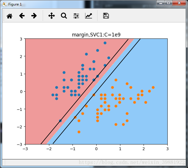
通过SVC1中的图，可以清晰的看出来，margin上边界有三个数据点落在直线上，下边界有两个数据点落在直线上，这些点就是支持向量，这种情况下相当于是硬间隔，在margin中间，没有任何数据点，既保证正确的将数据点分成了两类，且让两类数据点离决策边界最近的数据点又尽可能的远。

在SVC2中，给了很大的容错空间，所以在图中，margin中包含了许多数据点，且错分了一个蓝色的数据点。

补充：

LinearSVC中，multi_class='ovr'代表二分类问题，多分类问题设置成multi_class='ovo';penalty='l2':采用L2范式进行正则化

支持向量机SVM----学习笔记二（代码实践一线性分类）

Scikit-learn中的SVM

猜你喜欢