机器学习原理与实战 | SVM（支持向量机）实践

%matplotlib inline
import matplotlib.pyplot as plt
import numpy as np

1. 二维SVM分类例子

from sklearn.datasets import make_blobs

X, y = make_blobs(n_samples=100, centers=2, 
                  random_state=0, cluster_std=0.3)
X.shape, y.shape

((100, 2), (100,))

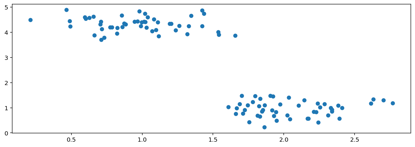
显示数据

plt.figure(figsize=(12, 4), dpi=144)
plt.scatter(X[:,0],X[:,1])

<matplotlib.collections.PathCollection at 0x18f06d80d08>

def plot_hyperplane(clf, X, y, 
                    h=0.02, 
                    draw_sv=True, 
                    title='hyperplan'):
    # create a mesh to plot in
    x_min, x_max = X[:, 0].min() - 1, X[:, 0].max() + 1
    y_min, y_max = X[:, 1].min() - 1, X[:, 1].max() + 1
    xx, yy = np.meshgrid(np.arange(x_min, x_max, h),
                         np.arange(y_min, y_max, h))

    plt.title(title)
    plt.xlim(xx.min(), xx.max())
    plt.ylim(yy.min(), yy.max())
    plt.xticks(())
    plt.yticks(())
    
    Z = clf.predict(np.c_[xx.ravel(), yy.ravel()])
    # Put the result into a color plot
    Z = Z.reshape(xx.shape)
    plt.contourf(xx, yy, Z, cmap='hot', alpha=0.5)

    markers = ['o', 's', '^']
    colors = ['b', 'r', 'c']
    labels = np.unique(y)
    for label in labels:
        plt.scatter(X[y==label][:, 0], 
                    X[y==label][:, 1], 
                    c=colors[label], 
                    marker=markers[label])
    if draw_sv:
        sv = clf.support_vectors_
        plt.scatter(sv[:, 0], sv[:, 1], c='y', marker='x')

from sklearn import svm
from sklearn.datasets import make_blobs

X, y = make_blobs(n_samples=100, centers=2, 
                  random_state=0, cluster_std=0.3)
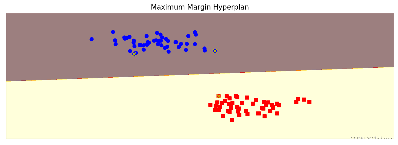
clf = svm.SVC(C=1.0, kernel='linear')
clf.fit(X, y)

plt.figure(figsize=(12, 4), dpi=144)
plot_hyperplane(clf, X, y, h=0.01, 
                title='Maximum Margin Hyperplan')

from sklearn import svm
from sklearn.datasets import make_blobs

X, y = make_blobs(n_samples=100, centers=3, 
                  random_state=0, cluster_std=0.8)

# 线性函数
clf_linear = svm.SVC(C=1.0, kernel='linear')
# 多项式核函数(3阶)
clf_poly = svm.SVC(C=1.0, kernel='poly', degree=3)
# 高斯核函数
clf_rbf = svm.SVC(C=1.0, kernel='rbf', gamma=0.5)
clf_rbf2 = svm.SVC(C=1.0, kernel='rbf', gamma=0.2)



plt.figure(figsize=(8, 5), dpi=100)

clfs = [clf_linear, clf_poly, clf_rbf, clf_rbf2]
titles = ['Linear Kernel', 
          'Polynomial Kernel with Degree=3', 
          'Gaussian Kernel with $\gamma=0.5$', 
          'Gaussian Kernel with $\gamma=0.1$']
for clf, i in zip(clfs, range(len(clfs))):
    clf.fit(X, y)
    plt.subplot(2, 2, i+1)
    plot_hyperplane(clf, X, y, title=titles[i])

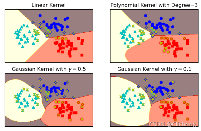
思考：左下角gamma=0.5的高斯核函数的图片，带有x标记的点是支持向量。我们之前介绍过，离分隔超平面最近的点是支持向量，为什么很多离分隔超平面很远的点，也是支持向量呢？

原因是高斯核函数把输入特征向量映射到了无限维的向量空间里，在映射后的高维向量空间里，这些点其实是离分隔超平面最近的点。当回到二维向量空间中时，这些点“看起来”就不像是距离分隔超平面最近的点了，但实际上它们就是支持向量。

2. 多维SVM分类例子

%matplotlib inline
import matplotlib.pyplot as plt
import numpy as np

# 载入数据
from sklearn.datasets import load_breast_cancer

cancer = load_breast_cancer()
X = cancer.data
y = cancer.target
print('data shape: {0}; no. positive: {1}; no. negative: {2}'.format(
    X.shape, y[y==1].shape[0], y[y==0].shape[0]))

data shape: (569, 30); no. positive: 357; no. negative: 212

切分数据集

from sklearn.model_selection import train_test_split

X_train, X_test, y_train, y_test = train_test_split(X, y, test_size=0.2)

2.1 高斯核函数

from sklearn.svm import SVC

clf = SVC(C=1.0, kernel='rbf', gamma=0.0001)
clf.fit(X_train, y_train)
train_score = clf.score(X_train, y_train)
test_score = clf.score(X_test, y_test)
print('train score: {0}; test score: {1}'.format(train_score, test_score))

train score: 0.9406593406593406; test score: 0.9649122807017544

可以使用前面介绍过的GridSearchCV来自动选择最优参数

from sklearn.model_selection import GridSearchCV

gammas = np.linspace(0, 0.0003, 30)
param_grid = {
    
    'gamma': gammas}
clf = GridSearchCV(SVC(), param_grid, cv=5)
clf.fit(X, y)
print("best param: {0}\nbest score: {1}".format(clf.best_params_,
                                                clf.best_score_))

# plt.figure(figsize=(10, 4), dpi=144)
# plot_param_curve(plt, gammas, clf.cv_results_, xlabel='gamma');

best param: {'gamma': 0.00011379310344827585}
best score: 0.9367334264865704

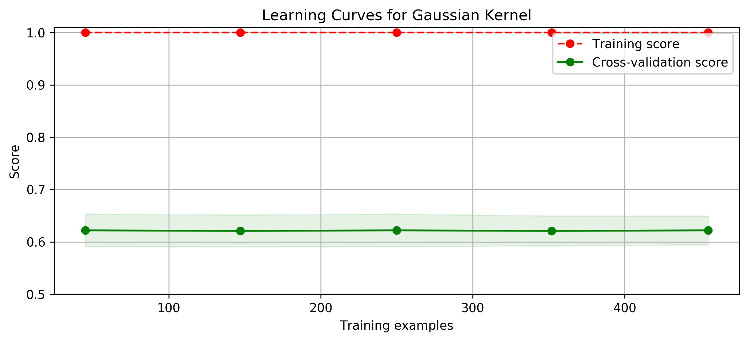
import time
from common.utils import plot_learning_curve
from sklearn.model_selection import ShuffleSplit

cv = ShuffleSplit(n_splits=10, test_size=0.2, random_state=0)
title = 'Learning Curves for Gaussian Kernel'

start = time.clock()
plt.figure(figsize=(10, 4), dpi=144)
plot_learning_curve(plt, SVC(C=1.0, kernel='rbf', gamma=0.01),
                    title, X, y, ylim=(0.5, 1.01), cv=cv)

print('elaspe: {0:.6f}'.format(time.clock()-start))

<Figure size 1440x576 with 0 Axes>
<module 'matplotlib.pyplot' from '/Users/kamidox/work/books/ml-scikit-learn/code/.venv/lib/python3.6/site-packages/matplotlib/pyplot.py'>
elaspe: 0.582505

2.2. 多项式核函数

from sklearn.svm import SVC

clf = SVC(C=1.0, kernel='poly', degree=2)
clf.fit(X_train, y_train)
train_score = clf.score(X_train, y_train)
test_score = clf.score(X_test, y_test)
print('train score: {0}; test score: {1}'.format(train_score, test_score))

/Users/kamidox/work/books/ml-scikit-learn/code/.venv/lib/python3.6/site-packages/sklearn/svm/base.py:196: FutureWarning: The default value of gamma will change from 'auto' to 'scale' in version 0.22 to account better for unscaled features. Set gamma explicitly to 'auto' or 'scale' to avoid this warning.
  "avoid this warning.", FutureWarning)

SVC(C=1.0, cache_size=200, class_weight=None, coef0=0.0,
  decision_function_shape='ovr', degree=2, gamma='auto_deprecated',
  kernel='poly', max_iter=-1, probability=False, random_state=None,
  shrinking=True, tol=0.001, verbose=False)

train score: 0.9802197802197802; test score: 0.9736842105263158

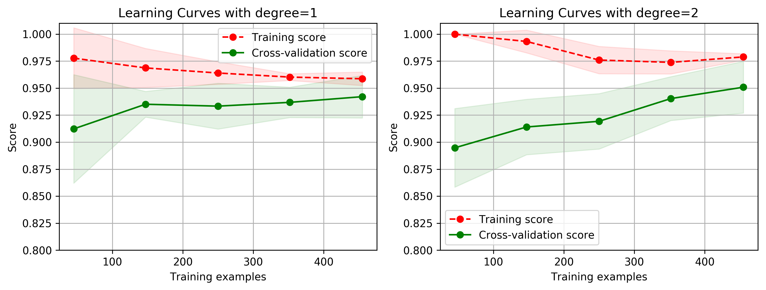
import time
from common.utils import plot_learning_curve
from sklearn.model_selection import ShuffleSplit

cv = ShuffleSplit(n_splits=5, test_size=0.2, random_state=0)
title = 'Learning Curves with degree={0}'
degrees = [1, 2]

start = time.clock()
plt.figure(figsize=(12, 4), dpi=144)
for i in range(len(degrees)):
    plt.subplot(1, len(degrees), i + 1)
    plot_learning_curve(plt, SVC(C=1.0, kernel='poly', degree=degrees[i]),
                        title.format(degrees[i]), X, y, ylim=(0.8, 1.01), cv=cv, n_jobs=4)

print('elaspe: {0:.6f}'.format(time.clock()-start))

<Figure size 1728x576 with 0 Axes>
elaspe: 0.260532

2.3 多项式 LinearSVC

from sklearn.svm import LinearSVC
from sklearn.preprocessing import PolynomialFeatures
from sklearn.preprocessing import MinMaxScaler
from sklearn.pipeline import Pipeline

def create_model(degree=2, **kwarg):
    polynomial_features = PolynomialFeatures(degree=degree,
                                             include_bias=False)
    scaler = MinMaxScaler()
    linear_svc = LinearSVC(**kwarg)
    pipeline = Pipeline([("polynomial_features", polynomial_features),
                         ("scaler", scaler),
                         ("linear_svc", linear_svc)])
    return pipeline


clf = create_model(penalty='l1', dual=False)
clf.fit(X_train, y_train)
train_score = clf.score(X_train, y_train)
test_score = clf.score(X_test, y_test)
print('train score: {0}; test score: {1}'.format(train_score, test_score))

/Users/kamidox/work/books/ml-scikit-learn/code/.venv/lib/python3.6/site-packages/sklearn/svm/base.py:922: ConvergenceWarning: Liblinear failed to converge, increase the number of iterations.
  "the number of iterations.", ConvergenceWarning)

Pipeline(memory=None,
     steps=[('polynomial_features', PolynomialFeatures(degree=2, include_bias=False, interaction_only=False)), ('scaler', MinMaxScaler(copy=True, feature_range=(0, 1))), ('linear_svc', LinearSVC(C=1.0, class_weight=None, dual=False, fit_intercept=True,
     intercept_scaling=1, loss='squared_hinge', max_iter=1000,
     multi_class='ovr', penalty='l1', random_state=None, tol=0.0001,
     verbose=0))])

train score: 0.9824175824175824; test score: 0.9912280701754386

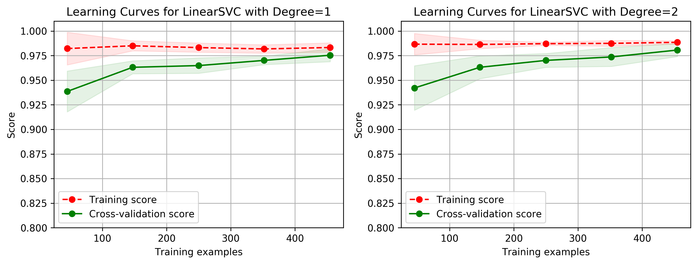
import time
from common.utils import plot_learning_curve
from sklearn.model_selection import ShuffleSplit

cv = ShuffleSplit(n_splits=5, test_size=0.2, random_state=0)
title = 'Learning Curves for LinearSVC with Degree={0}'
degrees = [1, 2]

start = time.clock()
plt.figure(figsize=(12, 4), dpi=144)
for i in range(len(degrees)):
    plt.subplot(1, len(degrees), i + 1)
    plot_learning_curve(plt, create_model(penalty='l1', dual=False, degree=degrees[i]),
                        title.format(degrees[i]), X, y, ylim=(0.8, 1.01), cv=cv)

print('elaspe: {0:.6f}'.format(time.clock()-start))

<Figure size 1728x576 with 0 Axes>
elaspe: 4.053868