Pytorch学习笔记(三) 图像分类器&数据并行处理

一、图像分类器

1.加载并处理输入数据

通常来说，处理图像、文本、语音或者视频数据时，可以使用标准 python 包将数据加载成 numpy 数组格式，然后将这个数组转换成 torch.*Tensor。

• 图像: Pillow，OpenCV
• 语音: scipy，librosa
• 文本: 可以直接用 Python 或 Cython 基础数据加载模块，或者 NLTK、SpaCy

几种常用数据集：CIFAR-10、ImageNet、MS-COCO、ImageFolder、LSUN Classification

torchvision: 含有支持加载类似Imagenet，CIFAR10，MNIST 等公共数据集的数据加载模块 torchvision.datasets 和支持加载图像数据数据转换模块 torch.utils.data.DataLoader

CIFAR-10: 32 * 32 * 3
包含十个类别: ‘airplane’, ‘automobile’, ‘bird’, ‘cat’, ‘deer’, ‘dog’, ‘frog’, ‘horse’, ‘ship’, ‘truck’

使用 .datasets.CIFAR10() 函数加载数据库。CIFAR-10有60000张图片，其中50000张是训练集，10000张是测试集。

torchvision里的数据集的输出是在[0, 1]范围内的PILImage图片，我们将他们转换成归一化范围为[-1,1]之间的 Tensors 。

关于数据预处理：归一化

import torch
import torchvision
import torchvision.transforms as transforms # transforms 用于数据预处理
# 数据预处理，帮助我们加快神经网络的训练
# compose函数将多个transforms包在一起
# transforms有许多种，例如transforms.ToTensor(),transforms.Scale()等
'''
1.ToTensor()是指把PIL.Image(RGB)或者numpy.ndarray(HxWxC)从0到255的值映射到0~1的范围内，并转化成Tensor格式.
2.Normalize(mean，std)是通过 channel=(channel-mean)/std 实现数据归一化.
'''
# 转换后，数据中的每个值就变成了[-1,1]的数了
transform=transforms.Compose(
    [transforms.ToTensor(),
     transforms.Normalize((0.5,0.5,0.5),(0.5,0.5,0.5))])

# 训练集，将相对目录./data下的cifar-10-batches-py文件夹中的全部数据（50000张图片作为训练数据）
# 加载到内存中，若download=True时，会自动从网上下载数据并解压
'''
root: 表示cifar10数据的加载的相对目录
train: 表示是否加载数据库的训练集，false的时候加载测试集
download: 表示是否自动下载cifar数据集
transform: 表示是否需要对数据进行预处理，none为不进行预处理
'''
trainset=torchvision.datasets.CIFAR10(root='./data',train=True,
                                      download=True,transform=transform)
# 我们在训练神经网络时，使用的是mini-batch（一次输入多张图片），
# 所以我们在使用一个叫DataLoader的工具将训练集的50000张图片划分成12500份数据包，每份4张图，用于mini-batch输入。
'''
shffule=True 在表示不同批次的数据遍历时，打乱顺序
num_workers=2表示使用两个子进程来加载数据
'''
trainloader=torch.utils.data.DataLoader(trainset,batch_size=4,
                                        shuffle=True,num_workers=2)
# print len(trainset) # 50000


testset=torchvision.datasets.CIFAR10(root='./data',train=False,
                                     download=True,transform=transform)
testloader=torch.utils.data.DataLoader(testset,batch_size=4,
                                       shuffle=False,num_workers=2)

classes =('plane','car','bird','cat',
          'deer','dog','frog','horse','ship','truck')
# Output: Files already downloaded and verified

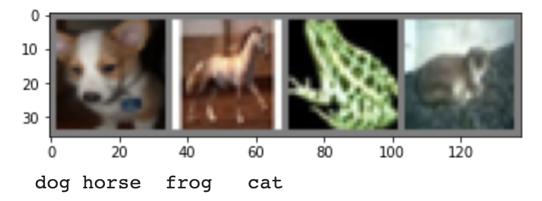
查看其中的部分数据

import matplotlib.pyplot as plt
import numpy as np

# functions to show an image
def imshow(img):
    img=img/2+0.5     # unnormalize
    npimg=img.numpy()
    plt.imshow(np.transpose(npimg, (1,2,0)))
    plt.show()

# get some random training images
dataiter=iter(trainloader)
images,labels=dataiter.next()

# show images
imshow(torchvision.utils.make_grid(images))
# print labels
print(' '.join('%5s' % classes[labels[j]] for j in range(4)))

2.训练和测试网络

训练的基本步骤：

1. 将 input 输入到 net 中，进行前向传播 forward() ，运算后得到output
2. 将 output 输入到选择的 loss function，计算loss值（标量）
3. 将梯度反向传播 backward() 到每个参数
4. 利用 new_w = pre_w + learning_rate * grad 进行权重更新

Pytorch中包括的各种 loss function
Pytorch官网 各种 Optimize 方法

import torch.nn as nn
import torch.nn.functional as F
import torch.optim as optim

class Net(nn.Module):
    def __init__(self):
        super(Net,self).__init__()
        self.conv1=nn.Conv2d(3,6,5)
        self.pool=nn.MaxPool2d(2,2)
        self.conv2=nn.Conv2d(6,16,5)
        self.fc1=nn.Linear(16*5*5,120)
        self.fc2=nn.Linear(120,84)
        self.fc3=nn.Linear(84,10)

    def forward(self, x):
        x=self.pool(F.relu(self.conv1(x)))
        x=self.pool(F.relu(self.conv2(x)))
        x=x.view(-1,16*5*5)
        x=F.relu(self.fc1(x))
        x=F.relu(self.fc2(x))
        x=self.fc3(x)
        return x

net = Net()
# 定义一个交叉熵损失函数 和 momentum SGD优化器
criterion=nn.CrossEntropyLoss()
optimizer=optim.SGD(net.parameters(),lr=0.001,momentum=0.9)

# 开始训练网络，只需要不断地迭代 不断通过输入进行参数调整
for epoch in range(2):  # loop over the dataset multiple times 定义迭代次数 即以不同数据顺序的数据集投入训练的次数

    running_loss=0.0 # 计算loss平均值
    for i,data in enumerate(trainloader,0):
        # get the inputs
        inputs,labels=data

        # zero the parameter gradients
        optimizer.zero_grad()

        # forward + backward + optimize
        outputs=net(inputs)
        loss=criterion(outputs,labels) # 使用输出值和真实值进行loss计算
        loss.backward() # 首先反向传播更新每一个网络参数的梯度
        optimizer.step() # 每个参数利用自身的梯度值进行梯度下降法的更新

        # print statistics
        running_loss+=loss.item()
        if i%2000==1999:    # print every 2000 mini-batches
            print('[%d, %5d] loss: %.3f' %
                  (epoch+1,i+1,running_loss/2000))
            running_loss=0.0

print('Finished Training')

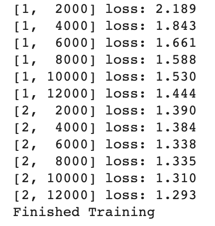
loss平均值每次跑都会有变化，因为 loader 设置了shuffle=True (在表示不同批次的数据遍历时，打乱顺序)

测试网络的准确度

correct=0
total=0
with torch.no_grad():
    for data in testloader:
        images,labels=data
        outputs=net(images)
        _,predicted=torch.max(outputs.data,dim=1) # dim=1表示输出所在行的最大值,dim=0则输出所在列的最大值
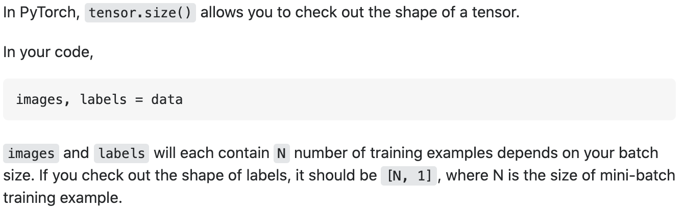
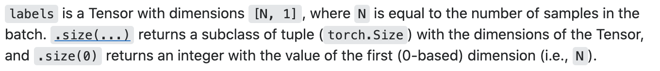
        total+=labels.size(0) # 我们的labels是4维的向量，size(0)就是4，即每次total都+4
        correct+=(predicted==labels).sum().item()

print('Accuracy of the network on the 10000 test images: %d %%' % (
    100*correct/total))
# Output: Accuracy of the network on the 10000 test images: 54%
# 随机预测的准确率为1/10=10%,所以网络的预测比随机预测要好，说明网络学到了东西

关于 labels.size(0)

关于 correct+=(predicted==labels).sum().item()

两个4维向量逐个对比，相同的记为1，不同的记为0，再利用 sum() 求各元素总和，得到相同的个数。

.sum() 之后得到的仍是tensor，要通过.item() 转换成数值。

import torch
import numpy as np
data1=np.array([
                [1,2,3],
                [4,5,6]
])
data1_t=torch.from_numpy(data1)
data2=np.array([
                [1,2,3],
                [1,5,8]
])
data2_t=torch.from_numpy(data1)
print(data1_t)
print(data2_t)
print(data1==data2)
'''
tensor([[1, 2, 3],
        [4, 5, 6]])
tensor([[1, 2, 3],
        [4, 5, 6]])
[[ True  True  True]
 [False  True False]]
'''

关于 _,predicted=torch.max(outputs.data,1) ：

outputs.data 是一个4x10张量，max函数会将每一行的最大的那一列的值和序号各自组成一个一维张量返回，第一个是值的张量，第二个是序号的张量。

import torch

data=torch.rand(4,10)
print(data)
print(torch.max(data,1)) # dim=1输出每行的最大值
print(torch.max(data,0)) # dim=0输出每列的最大值
'''
tensor([[0.4970, 0.0473, 0.4645, 0.9327, 0.7883, 0.6930, 0.0298, 0.6272, 0.4781,
         0.4188],
        [0.7484, 0.8171, 0.6512, 0.0057, 0.0043, 0.3213, 0.2929, 0.6281, 0.5625,
         0.0521],
        [0.4678, 0.1851, 0.8253, 0.0938, 0.2897, 0.8337, 0.7507, 0.0200, 0.2184,
         0.1595],
        [0.6984, 0.8119, 0.2741, 0.2171, 0.5258, 0.4051, 0.4047, 0.4991, 0.3526,
         0.1946]])

torch.return_types.max(
values=tensor([0.9327, 0.8171, 0.8337, 0.8119]),
indices=tensor([3, 1, 5, 1]))

torch.return_types.max(
values=tensor([0.7484, 0.8171, 0.8253, 0.9327, 0.7883, 0.8337, 0.7507, 0.6281, 0.5625,
        0.4188]),
indices=tensor([1, 1, 2, 0, 0, 2, 2, 1, 1, 0]))
'''

分类测试准确度

list(0. for i in range(10)): 列表解析式

torch.squeeze() 和torch.unsqueeze()的用法

class_correct=list(0. for i in range(10)) # 清零
class_total=list(0. for i in range(10))
with torch.no_grad():
    for data in testloader:
        images,labels=data
        outputs=net(images)
        _,predicted=torch.max(outputs,1)
        c=(predicted==labels).squeeze()
        for i in range(4):
            label=labels[i]
            class_correct[label]+=c[i].item()
            class_total[label]+=1

for i in range(10):
    print('Accuracy of %5s : %2d%%' % (
        classes[i],100*class_correct[i]/class_total[i]))
'''
Accuracy of plane : 44%
Accuracy of   car : 70%
Accuracy of  bird : 31%
Accuracy of   cat : 32%
Accuracy of  deer : 46%
Accuracy of   dog : 60%
Accuracy of  frog : 65%
Accuracy of horse : 61%
Accuracy of  ship : 74%
Accuracy of truck : 62%
'''        

学习参考链接
PyTorch官方教程中文版

3.在GPU上训练

# 检查是否有可用的 GPU 来训练
device = torch.device("cuda:0" if torch.cuda.is_available() else "cpu")
print(device)
# 将网络参数和数据都转移到 GPU 上
net.to(device)
inputs,labels=inputs.to(device),labels.to(device) # 必须在每一个步骤向GPU发送输入数据和目标数据 

修改后的训练代码

import time
device=torch.device("cuda:0" if torch.cuda.is_available() else "cpu")
# 在 GPU 上训练注意需要将网络和数据放到 GPU 上
net.to(device)
criterion=nn.CrossEntropyLoss()
optimizer=optim.SGD(net.parameters(),lr=0.001,momentum=0.9)

start=time.time()
for epoch in range(2):

    running_loss=0.0
    for i, data in enumerate(trainloader,0):
        # 获取输入数据
        inputs,labels=data
        inputs,labels=inputs.to(device),labels.to(device)
        # 清空梯度缓存
        optimizer.zero_grad()

        outputs=net(inputs)
        loss=criterion(outputs,labels)
        loss.backward()
        optimizer.step()

        # 打印统计信息
        running_loss+=loss.item()
        if i%2000==1999:
            # 每 2000 次迭代打印一次信息
            print('[%d, %5d] loss: %.3f' % (epoch + 1, i+1, running_loss / 2000))
            running_loss=0.0
print('Finished Training! Total cost time: ', time.time() - start)

二、数据并行处理

DataParallel 会自动分割数据集并发送任务给多个 GPUs 上的多个模型，然后等待每个模型都完成各自的工作后，它又会收集并融合结果，再返回。

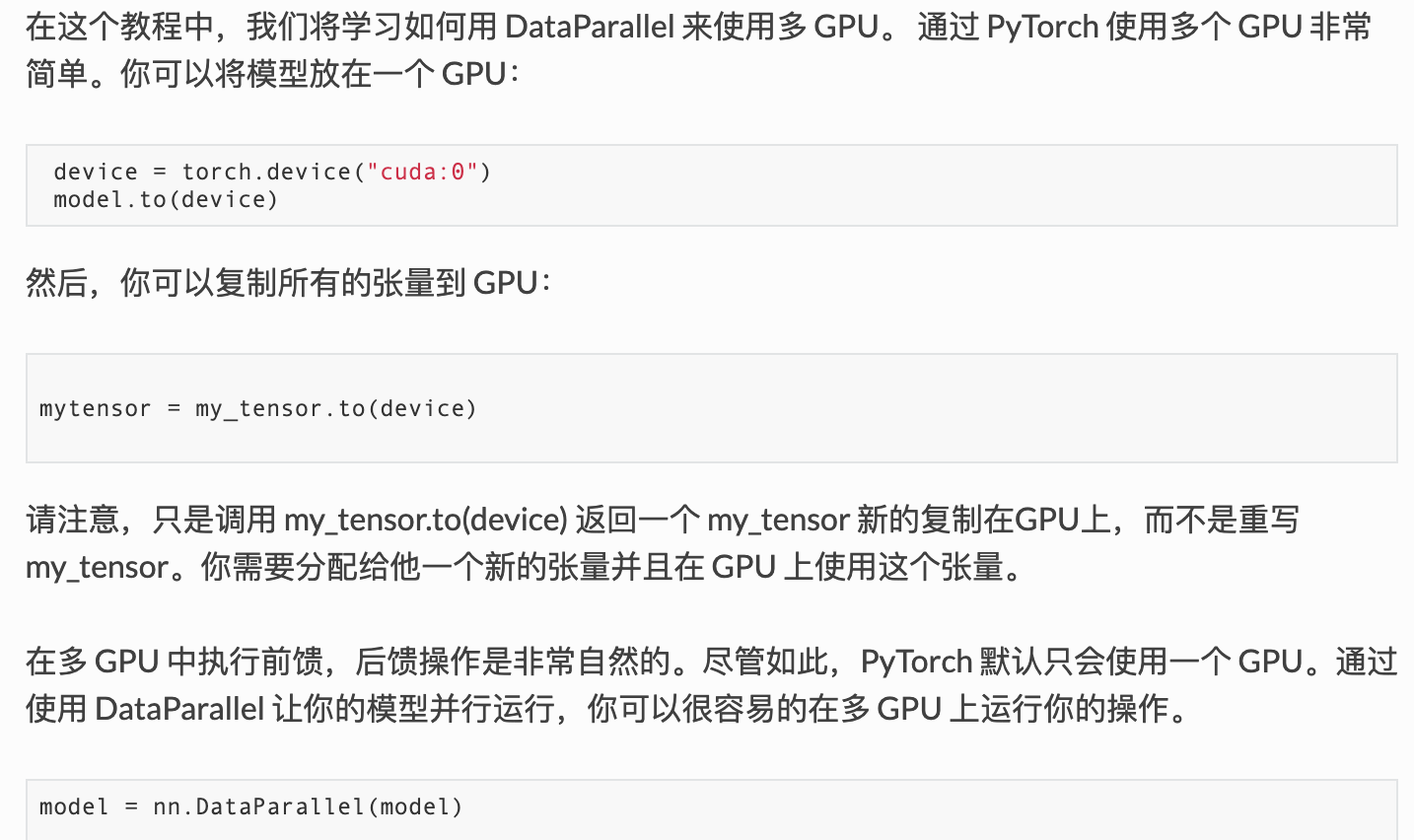
#device = torch.device("cuda:0")
#model.to(device)

#mytensor = my_tensor.to(device)
#model = nn.DataParallel(model)

import torch
import torch.nn as nn
from torch.utils.data import Dataset, DataLoader

# Parameters and DataLoaders
input_size = 5
output_size = 2

batch_size = 30
data_size = 100

device = torch.device("cuda:0" if torch.cuda.is_available() else "cpu")
class RandomDataset(Dataset):

    def __init__(self, size, length):
        self.len = length
        self.data = torch.randn(length, size)

    def __getitem__(self, index):
        return self.data[index]

    def __len__(self):
        return self.len

rand_loader = DataLoader(dataset=RandomDataset(input_size, data_size),batch_size=batch_size, shuffle=True)

class Model(nn.Module):
    # Our model

    def __init__(self, input_size, output_size):
        super(Model, self).__init__()
        # 构建一个简单的网络模型，仅仅包含一层全连接层的神经网络
        self.fc = nn.Linear(input_size, output_size) 

    def forward(self, input):
        output = self.fc(input)
        # 监控网络输入和输出tensors的大小：
        print("\tIn Model: input size", input.size(),
              "output size", output.size())

        return output

# 创建模型并且数据并行处理 (核心)
# 首先需要定义一个模型实例
model = Model(input_size, output_size)
# 检查是否拥有多个 GPUs，如果是就可以将模型包裹在 nn.DataParallel ，并调用 model.to(device) 。
if torch.cuda.device_count() > 1:
  print("Let's use", torch.cuda.device_count(), "GPUs!")
  # dim = 0 [30, xxx] -> [10, ...], [10, ...], [10, ...] on 3 GPUs
  model = nn.DataParallel(model)

model.to(device)
# 运行模型，看看打印的信息
for data in rand_loader:
    input = data.to(device)
    output = model(input)
    print("Outside: input size", input.size(),
          "output_size", output.size())

如果仅仅只有 1 个或者没有 GPU ，那么 batch=30 的时候，模型会得到输入输出的大小都是 30。

In Model: input size torch.Size([30, 5]) output size torch.Size([30, 2])
Outside: input size torch.Size([30, 5]) output_size torch.Size([30, 2])
	In Model: input size torch.Size([30, 5]) output size torch.Size([30, 2])
Outside: input size torch.Size([30, 5]) output_size torch.Size([30, 2])
	In Model: input size torch.Size([30, 5]) output size torch.Size([30, 2])
Outside: input size torch.Size([30, 5]) output_size torch.Size([30, 2])
	In Model: input size torch.Size([10, 5]) output size torch.Size([10, 2])
Outside: input size torch.Size([10, 5]) output_size torch.Size([10, 2])

# on 2 GPUs
Let's use 2 GPUs!
    In Model: input size torch.Size([15, 5]) output size torch.Size([15, 2])
    In Model: input size torch.Size([15, 5]) output size torch.Size([15, 2])
Outside: input size torch.Size([30, 5]) output_size torch.Size([30, 2])
    In Model: input size torch.Size([15, 5]) output size torch.Size([15, 2])
    In Model: input size torch.Size([15, 5]) output size torch.Size([15, 2])
Outside: input size torch.Size([30, 5]) output_size torch.Size([30, 2])
    In Model: input size torch.Size([15, 5]) output size torch.Size([15, 2])
    In Model: input size torch.Size([15, 5]) output size torch.Size([15, 2])
Outside: input size torch.Size([30, 5]) output_size torch.Size([30, 2])
    In Model: input size torch.Size([5, 5]) output size torch.Size([5, 2])
    In Model: input size torch.Size([5, 5]) output size torch.Size([5, 2])
Outside: input size torch.Size([10, 5]) output_size torch.Size([10, 2])

Let's use 3 GPUs!
    In Model: input size torch.Size([10, 5]) output size torch.Size([10, 2])
    In Model: input size torch.Size([10, 5]) output size torch.Size([10, 2])
    In Model: input size torch.Size([10, 5]) output size torch.Size([10, 2])
Outside: input size torch.Size([30, 5]) output_size torch.Size([30, 2])
    In Model: input size torch.Size([10, 5]) output size torch.Size([10, 2])
    In Model: input size torch.Size([10, 5]) output size torch.Size([10, 2])
    In Model: input size torch.Size([10, 5]) output size torch.Size([10, 2])
Outside: input size torch.Size([30, 5]) output_size torch.Size([30, 2])
    In Model: input size torch.Size([10, 5]) output size torch.Size([10, 2])
    In Model: input size torch.Size([10, 5]) output size torch.Size([10, 2])
    In Model: input size torch.Size([10, 5]) output size torch.Size([10, 2])
Outside: input size torch.Size([30, 5]) output_size torch.Size([30, 2])
    In Model: input size torch.Size([4, 5]) output size torch.Size([4, 2])
    In Model: input size torch.Size([4, 5]) output size torch.Size([4, 2])
    In Model: input size torch.Size([2, 5]) output size torch.Size([2, 2])
Outside: input size torch.Size([10, 5]) output_size torch.Size([10, 2])

Let's use 8 GPUs!
    In Model: input size torch.Size([4, 5]) output size torch.Size([4, 2])
    In Model: input size torch.Size([4, 5]) output size torch.Size([4, 2])
    In Model: input size torch.Size([2, 5]) output size torch.Size([2, 2])
    In Model: input size torch.Size([4, 5]) output size torch.Size([4, 2])
    In Model: input size torch.Size([4, 5]) output size torch.Size([4, 2])
    In Model: input size torch.Size([4, 5]) output size torch.Size([4, 2])
    In Model: input size torch.Size([4, 5]) output size torch.Size([4, 2])
    In Model: input size torch.Size([4, 5]) output size torch.Size([4, 2])
Outside: input size torch.Size([30, 5]) output_size torch.Size([30, 2])
    In Model: input size torch.Size([4, 5]) output size torch.Size([4, 2])
    In Model: input size torch.Size([4, 5]) output size torch.Size([4, 2])
    In Model: input size torch.Size([4, 5]) output size torch.Size([4, 2])
    In Model: input size torch.Size([4, 5]) output size torch.Size([4, 2])
    In Model: input size torch.Size([4, 5]) output size torch.Size([4, 2])
    In Model: input size torch.Size([4, 5]) output size torch.Size([4, 2])
    In Model: input size torch.Size([2, 5]) output size torch.Size([2, 2])
    In Model: input size torch.Size([4, 5]) output size torch.Size([4, 2])
Outside: input size torch.Size([30, 5]) output_size torch.Size([30, 2])
    In Model: input size torch.Size([4, 5]) output size torch.Size([4, 2])
    In Model: input size torch.Size([4, 5]) output size torch.Size([4, 2])
    In Model: input size torch.Size([4, 5]) output size torch.Size([4, 2])
    In Model: input size torch.Size([4, 5]) output size torch.Size([4, 2])
    In Model: input size torch.Size([4, 5]) output size torch.Size([4, 2])
    In Model: input size torch.Size([4, 5]) output size torch.Size([4, 2])
    In Model: input size torch.Size([4, 5]) output size torch.Size([4, 2])
    In Model: input size torch.Size([2, 5]) output size torch.Size([2, 2])
Outside: input size torch.Size([30, 5]) output_size torch.Size([30, 2])
    In Model: input size torch.Size([2, 5]) output size torch.Size([2, 2])
    In Model: input size torch.Size([2, 5]) output size torch.Size([2, 2])
    In Model: input size torch.Size([2, 5]) output size torch.Size([2, 2])
    In Model: input size torch.Size([2, 5]) output size torch.Size([2, 2])
    In Model: input size torch.Size([2, 5]) output size torch.Size([2, 2])
Outside: input size torch.Size([10, 5]) output_size torch.Size([10, 2])

参考链接：

知乎版60min入门解读

Pytorch中文官网

Pytoch英文版

更详细的数据并行处理教程