PyTorch学习之 图像分类器
学习网站
http://pytorch123.com/SecondSection/neural_networks/
训练一个图像分类器
通过前面的章节,我们已经知道怎样定义一个神经网络,以及计算其损失函数,并且更新网络的权重
现在,我们将要学习怎样去处理数据。
一般来说,当处理图像,文本,音频,视频这些数据时,可以使用标准的python包来下载这些数据,
并转换成numpy数组格式。然后,将这些数组转换成 “torch.Tensor”格式
- 对于图像,可以使用Pillow,OpenCV包
- 对于音频,可以使用 scipy, librosa包
- 对于文本,可以使用Python或者Cyphon直接加载,或者使用NLTK和SpaCy
对于视觉,PytorCh中创建了一个“torchvision”包,里面包含一些常见的数据集,例如
Imagenet, CIFAR10, MNIST等,以及一些图像转换模块:torchvision.datasets, torch.utils.data.DataLoader
下面会使用CIFAR10数据集作为例子,进行图像分类:
CIFAR10: ‘airplane’, ‘automobile’, ‘bird’, ‘cat’, ‘deer’,‘dog’, ‘frog’, ‘horse’, ‘ship’, ‘truck’.
尺寸:3*32*32
图像分类一般分为以下5个步骤
- 使用torchvision加载并且归一化CIFAR10的训练和测试数据集
- 定义一个卷积神经网络
- 定义一个损失函数
- 在训练样本数据上训练网络
- 在测试样本数据上测试网络
1. 下载并归一化CIFAR10数据集
import torch
import torchvision
import torchvision.transforms as transforms

########################################################################
# torchvision加载的数据都是PILImage的数据类型,在[0, 1]之间
# 对上述类型的数据集进行归一化为[-1, 1]范围的tensors
# 归一化方法: (X-mean)/std
transform = transforms.Compose(
    [transforms.ToTensor(),
     transforms.Normalize((0.5, 0.5, 0.5), (0.5, 0.5, 0.5))]) # mean, std
# 检验是否已经存在,若不存在,则下载数据集
trainset = torchvision.datasets.CIFAR10(root='./data', train=True,
                                        download=True, transform=transform)
# 数据加载器,结合了数据集和取样器,并且可以提供多个线程处理数据集。
# 在训练模型时使用到此函数,用来把训练数据分成多个小组,此函数每次抛出一组数据。
# 直至把所有的数据都抛出。就是做一个数据的初始化。
trainloader = torch.utils.data.DataLoader(trainset, batch_size=4,
                                          shuffle=True, num_workers=0)

testset = torchvision.datasets.CIFAR10(root='./data', train=False,
                                       download=True, transform=transform)
testloader = torch.utils.data.DataLoader(testset, batch_size=4,
                                         shuffle=False, num_workers=0)

classes = ('plane', 'car', 'bird', 'cat',
           'deer', 'dog', 'frog', 'horse', 'ship', 'truck')
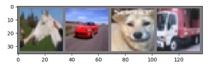
显示数据中的一些图像
########################################################################
# 显示数据集中的一些图像

import matplotlib.pyplot as plt
import numpy as np

def imshow(img):
    img = img / 2 + 0.5     # unnormalize, 因为前面是将图像进行了归一化,即 x = (X-0.5)/0.5
    npimg = img.numpy()
    image = np.transpose(npimg, (1, 2, 0))
    plt.imshow(image)    # 1 是和第二个轴交换,2,是和第2个轴交换,0是和第一个轴交换image[Height, Width, Dim]
    plt.show()

# get some random training images
dataiter = iter(trainloader)     # 使得 trainloader 变成迭代器
images, labels = dataiter.next()

# show images
imshow(torchvision.utils.make_grid(images))  # 将若干图像拼成一幅图像
# print labels
print(' '.join('%5s' % classes[labels[j]] for j in range(4)))
2. 定义一个卷积神经网络
import torch.nn as nn
import torch.nn.functional as F

class Net(nn.Module):
    def __init__(self):
        super(Net, self).__init__()
        self.conv1 = nn.Conv2d(3, 6, 5)   # 输出 6*28*28
        self.pool = nn.MaxPool2d(2, 2)    # 6*14*14
        self.conv2 = nn.Conv2d(6, 16, 5)  # 16*10*10
        self.fc1 = nn.Linear(16 * 5 * 5, 120)  # conv2经过 pooling 后,变成 5*5 map, 所以 16*5*5个全连接神经元
        self.fc2 = nn.Linear(120, 84)
        self.fc3 = nn.Linear(84, 10)

    def forward(self, x):
        x = self.pool(F.relu(self.conv1(x)))   # 卷积 -> Relu -> Pool
        x = self.pool(F.relu(self.conv2(x)))
        x = x.view(-1, 16 * 5 * 5)             # view函数将张量x变形成一维的向量形式,作为全连接的输入
        x = F.relu(self.fc1(x))
        x = F.relu(self.fc2(x))
        x = self.fc3(x)
        return x

net = Net()
3. 定义损失函数与优化器
import torch.optim as optim

criterion = nn.CrossEntropyLoss()  # 损失函数
optimizer = optim.SGD(net.parameters(), lr=0.001, momentum=0.9)  # 优化器 SGD with momentum
4. 训练网络
for epoch in range(2):  # 训练集训练次数

    running_loss = 0.0
    # enumerate()用于可迭代\可遍历的数据对象组合为一个索引序列,
    # 同时列出数据和数据下标.上面代码的0表示从索引从0开始,
    for i, data in enumerate(trainloader, 0):
        # 获得输入
        inputs, labels = data
        # 初始化参数梯度
        optimizer.zero_grad()
        # 前馈 + 后馈 + 优化
        outputs = net(inputs)
        loss = criterion(outputs, labels)    # labels 会进行二值化,即[1 0 0 0 0 0 0 0 0]
        loss.backward()    # 梯度反向传播
        optimizer.step()   # 更新参数空间

        # print statistics
        running_loss += loss.item()
        if i % 2000 == 1999:    # print every 2000 mini-batches
            print('[%d, %5d] loss: %.3f' %
                  (epoch + 1, i + 1, running_loss / 2000))
            running_loss = 0.0

print('Finished Training')
5. 在数据集上测试网络结构
上面已经在训练集上进行了2次完整的训练循环,但是我们需要检查网络是否真正的学到了一些什么东西。测试的方式是,将网络输出的结果与数据集的ground-truth进行对比.
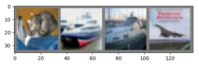
- 首先,显示一些图像
dataiter = iter(testloader)
images, labels = dataiter.next()
# 输出图像
imshow(torchvision.utils.make_grid(images))
print('GroundTruth: ', ' '.join('%5s' % classes[labels[j]] for j in range(4)))
print :
GroundTruth:    cat  ship  ship plane
- 查看网络输出结果
outputs = net(images)
outputs
tensor([[-1.3145, -2.4341, -0.7362,  6.8300,  0.5993,  2.2841, -0.9894, -0.9424,
          1.3211, -3.0649],
        [ 4.2055,  8.5567, -2.8397, -2.3198, -3.1733, -4.6069, -8.4125, -2.9534,
         10.5395,  5.7375],
        [ 1.3612,  1.1350,  0.3872, -0.3729, -0.1908, -1.1665, -3.7862, -0.3712,
          3.3340, -0.1305],
outputs 是10种类别分别预测出来的能量值,即某一类的能量值越高,其被认为是该种类的概率越大。因此,我们需要获得outputs中类被能量的最大值所对应的种类。
_, predicted = torch.max(outputs, 1)   # predicted 对应的种类
print('Predicted: ', ' '.join('%5s' % classes[predicted[j]]
                              for j in range(4)))
Predicted:    cat  ship  ship  ship
tensor([3, 8, 8, 8])
从上面的输出结果看,检测结果似乎还是不错的。
下面,我们看一下训练的网络在整个数据集上的表现。
correct = 0   #预测正确的数据
total = 0     #总共的数据
with torch.no_grad():     # 因为是进行测试,所以不需要进行梯度传播
    for data in testloader:
        images, labels = data
        outputs = net(images)   #输出结果
        _, predicted = torch.max(outputs.data, 1) #选择数值最大的一类作为其预测结果
        total += labels.size(0)
        correct += (predicted == labels).sum().item()   # 预测值与标签相同则预测正确

print('Accuracy of the network on the 10000 test images: %d %%' % (
    100 * correct / total))
Accuracy of the network on the 10000 test images: 55 %
因为随机预测的概率是10%(10类中预测一类),所以55%看起来要比随机预测好很多,似乎学到了一些东西。
下面,我们来进一步看一下,哪些类的预测比较好一些,哪些表现的不好。
class_correct = list(0. for i in range(10))
class_total = list(0. for i in range(10))
with torch.no_grad():
    for data in testloader:
        images, labels = data
        outputs = net(images)
        _, predicted = torch.max(outputs, 1)
        c = (predicted == labels).squeeze()   # 将shape中为1的维度去掉
        for i in range(4):
            label = labels[i]
            class_correct[label] += c[i].item()   # 正确预测累计
            class_total[label] += 1               # 每一类的总数

for i in range(10):
    print('Accuracy of %5s : %2d %%' % (
        classes[i], 100 * class_correct[i] / class_total[i]))   # 每一类的准确率
Accuracy of plane : 52 %
Accuracy of   car : 70 %
Accuracy of  bird : 44 %
Accuracy of   cat : 28 %
Accuracy of  deer : 54 %
Accuracy of   dog : 41 %
Accuracy of  frog : 66 %
Accuracy of horse : 60 %
Accuracy of  ship : 65 %
Accuracy of truck : 68 %
6. 在GPU上训练数据
在GPU上训练神经网络,就像将一个Tensor转移到GPU上一样。
首先来定义我们的device作为第一个可见的cuda device。
device = torch.device("cuda:0" if torch.cuda.is_available() else "cpu")
# 如果程序运行在CUDA机器上,下面会输出一个device的id
print(device)
cuda:0
设定好之后,这些方法就会递归的遍历所有模块,并把他们的参数和buffers转换为cuda的tensors
下面的语句是必不可少的:
net.to(device)
同时,也必须每一个步骤都要向gpu中发送inputs和targets.
inputs, labels = inputs.to(device), labels.to(device)
当网络非常小的时候,感觉不带速度的变化,可以把卷积1的输出改为128,卷积2的输入改为128,观察效果。改为128后,训练2次后的准确率为
Accuracy of the network on the 10000 test images: 60 %
更多的特征图的结果似乎要比6个特征图要好一些,下面是每个类的输出结果
Accuracy of plane : 73 %
Accuracy of   car : 82 %
Accuracy of  bird : 27 %
Accuracy of   cat : 32 %
Accuracy of  deer : 53 %
Accuracy of   dog : 55 %
Accuracy of  frog : 75 %
Accuracy of horse : 76 %
Accuracy of  ship : 70 %
Accuracy of truck : 54 %
备注:
改成GPU运行方式后会出现如下报错:
TypeError: can't convert CUDA tensor to numpy. Use Tensor.cpu() to copy the tensor to host memory first.
解决方法:
将 npimg = img.numpy() 改为
npimg = img.cpu().numpy()
