【Tensorflow】交叉熵数据验证（上）---CategoricalCrossentropy多分类

every blog every motto: You can do more than you think.

0. 前言

对（CategoricalCrossentropy多分类）交叉熵的具体过程用数据进行验证
说明： 后面总结部分更加直观

1. 正文

1.1 基本概念

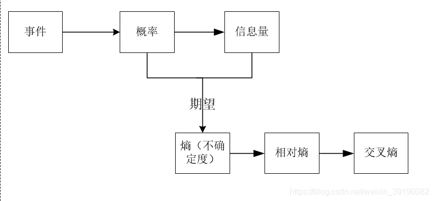
1.1.1 信息量

信息量用来衡量一个事件的不确定性。

1. 事件发生概率越大，(不确定性越小）其所含信息越小。
2. 事件发生概率越小，（不确定性越低）其所含信息越大。

例子：

• 太阳从东边升起（发生概率大，信息少）
• 月球有生物（发生概率小，信息大）
• 中国队进世界杯决赛（发生概率低，信息大）

---

由上面我们知道，信息量可由事件发生的概率进行刻画，如：
假设x是一个离散型随机变量，其取值集合为x,概率分布函数为p(x)=P(X=x)，则其可定义事件X=x0的信息量为：

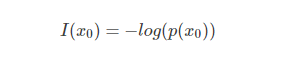
概率取值范围为（0~1），如下图：

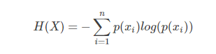
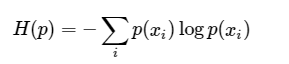
1.1.2 熵

事件	概率	信息量
A明天晴天	0.7	-log(p(A))=0.36
B明天下雨	0.2	-log(p(B))=1.61
C明天下雪	0.1	-log(p(C ))=2.30

熵：表示所有信息量的期望。

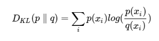
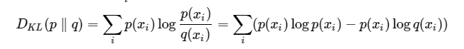
1.1.3 相对熵（KL散度）

相对熵（KL散度）：对于同一个随机变量x有两个单独的概率分布P（x）和Q（x），我们可以使用相对熵来衡量二者的差异

相对熵性质：

• 如果P和Q的分布相同，则相对熵为0
• D（p|q）和D（q|p）不相等，即，相对熵不具有对称性
• D（p|q）大于等于0

---

相对熵是用来衡量同一个随机变量的两个分布之间的距离，即机器学习中，p(x)是目标（标签）分布，q(x）是预测分布，为了让两个分布尽可能的接近，则需要相对熵尽可能的小。

1.1.4 交叉熵

相对熵：

目标事件的熵（信息量的期望）：

推演：

即：
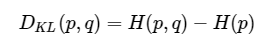
相对熵 = 交叉熵+事件P的熵

---

在机器学习中，目标事件P是我们的训练数据，即H ( p ) 是一个常量，则，最小化相对熵和最小化交叉熵等价

1.2 数据验证

导入库

import os

os.environ['TF_CPP_MIN_LOG_LEVEL'] = '2'
import tensorflow as tf
from tensorflow.keras.losses import CategoricalCrossentropy, BinaryCrossentropy
import numpy as np

loss = CategoricalCrossentropy()

1.2.1 一维

# 一维
p = np.array([1, 0, 0])
q = np.array([0.7, 0.2, 0.1])

1. 交叉熵函数：

# 1. 交叉熵
loss_result_1 = loss(p, q)
print('交叉熵计算:', loss_result_1)

2. numpy计算

# 2. numpy计算
np_result_1 = p * np.log(q)
np_result_1 = -np.sum(np_result_1)
print('numpy计算:', np_result_1)

3. 逐个元素计算

# 3. 单个元素计算
s_1 = 1 * np.log(0.7)
s_2 = 0 * np.log(0.2)
s_3 = 0 * np.log(0.1)
print('s_1:', s_1, '; s_2:', s_2, '; s_3:', s_3)
single_result_1 = -(s_1 + s_2 + s_3)
print('单独计算：', single_result_1)

---

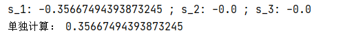
三者结果：

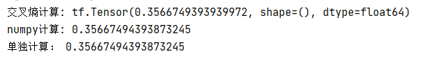
小结： 三者计算结果并没有差别

1.2.2 二维

# 二维
p = np.array([[1, 0, 0], [1, 0, 0]])
q = np.array([[0.7, 0.2, 0.1], [0.8, 0.1, 0.1]])

print(p.shape)
print(q.shape)

print('p:\n', p)
print('q:\n', q)

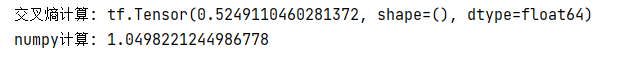
1. 交叉熵函数

# 1. 交叉熵
loss_result_1 = loss(p, q)
print('交叉熵计算:', loss_result_1)

2. numpy计算

# 2. numpy计算
np_result_1 = p * np.log(q)
np_result_1 = -np.sum(np_result_1)
print('numpy计算:', np_result_1)

3. 单个元素计算

# 3. 单个元素计算
s_1_1 = 1 * np.log(0.7)
s_1_2 = 0 * np.log(0.2)
s_1_3 = 0 * np.log(0.1)
s_2_1 = 1 * np.log(0.8)
s_2_2 = 0 * np.log(0.1)
s_2_3 = 0 * np.log(0.1)
print('s_1_1:', s_1_1)
print('s_1_2:', s_1_2)
print('s_1_3:', s_1_3)
print('s_2_1:', s_2_1)
print('s_2_2:', s_2_2)
print('s_2_3:', s_2_3)
single_result_1 = -(s_1_1 + s_1_2 + s_1_3 + s_2_1 + s_2_2 + s_2_3)
print('单独计算：', single_result_1)

---

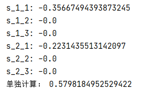
三者结果：

小结： numpy计算结果和逐个元素计算结果相同，但和交叉熵函数计算结果不同（后面解释）

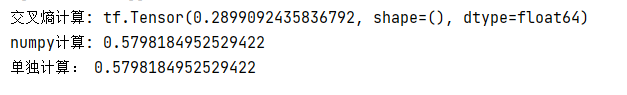
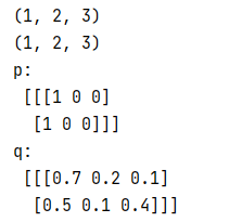
1.2.3 三维

# 三维
p = np.array([[[1, 0, 0], [1, 0, 0]]])
q = np.array([[[0.7, 0.2, 0.1], [0.5, 0.1, 0.4]]])

print(p.shape)
print(q.shape)
print('p:\n', p)
print('q:\n', q)

# 1. 交叉熵
loss_result_1 = loss(p, q)
print('交叉熵计算:', loss_result_1)
# 2. numpy计算
np_result_1 = p * np.log(q)
np_result_1 = -np.sum(np_result_1)
print('numpy计算:', np_result_1)

小结： 元素较多，故省略逐元素计算；前面我们已经发现，逐元素计算和我们的numpy计算结果一样，后续一并省略逐元素计算。

1.2.4 四维

p = np.array([
    [[[1, 0, 0], [1, 0, 0], [0, 0, 1], [0, 0, 1]],
     [[1, 0, 0], [1, 0, 0], [0, 0, 1], [0, 0, 1]],
     [[1, 0, 0], [1, 0, 0], [0, 0, 1], [0, 0, 1]], ],
    [[[1, 0, 0], [1, 0, 0], [0, 0, 1], [0, 0, 1]],
     [[1, 0, 0], [1, 0, 0], [0, 0, 1], [0, 0, 1]],
     [[1, 0, 0], [1, 0, 0], [0, 0, 1], [0, 0, 1]], ]

])
q = np.array([
    [[[0.7, 0.2, 0.1], [0.8, 0.1, 0.1], [0.2, 0.2, 0.6], [0.1, 0.2, 0.7]],
     [[0.7, 0.2, 0.1], [0.8, 0.1, 0.1], [0.2, 0.2, 0.6], [0.1, 0.2, 0.7]],
     [[0.7, 0.2, 0.1], [0.8, 0.1, 0.1], [0.2, 0.2, 0.6], [0.1, 0.2, 0.7]], ],
    [[[0.7, 0.2, 0.1], [0.8, 0.1, 0.1], [0.2, 0.2, 0.6], [0.1, 0.2, 0.7]],
     [[0.7, 0.2, 0.1], [0.8, 0.1, 0.1], [0.2, 0.2, 0.6], [0.1, 0.2, 0.7]],
     [[0.7, 0.2, 0.1], [0.8, 0.1, 0.1], [0.2, 0.2, 0.6], [0.1, 0.2, 0.7]], ]

])
print(p.shape)
print(q.shape)

# 1. 交叉熵
loss_result_1 = loss(p, q)
print('交叉熵计算:', loss_result_1)
# 2. numpy计算
np_result_1 = p * np.log(q)
np_result_1 = -np.sum(np_result_1)
print('numpy计算:', np_result_1)

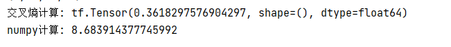
说明： 在tensorflow中默认执行的值channel_last，即四维：（batch,height,widht,channel）

1.2.5 小结

如下是一张（1，2，2，2）的图片：
说明： shape:（batch,height,widht,channel）,可以把通道（最后一维）理解为上下叠加的图层或上下叠加的大饼。

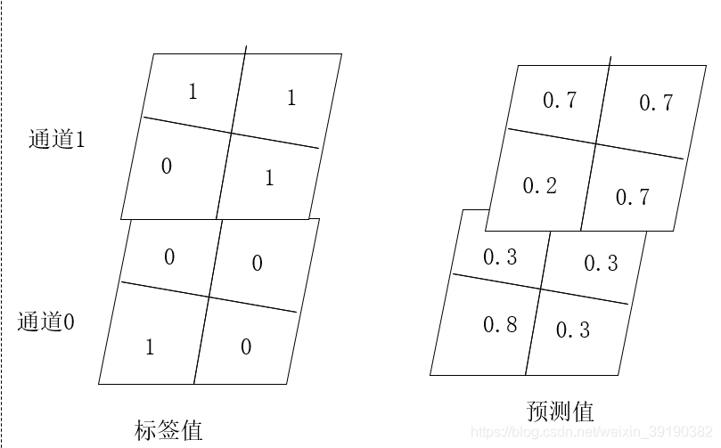
p = np.array([[[[0, 1], [0, 1]], [[1, 0], [0, 1]]]])
print(p[:, :, :, 0])
print(p[:, :, :, 1])
print('----------')
q = np.array([[[[0.3, 0.7], [0.3, 0.7]], [[0.8, 0.2], [0.3, 0.7]]]])
print(q[..., 0])
print(q[..., 1])

print(p.shape)
print(q.shape)
# 1. 交叉熵
loss_result_1 = loss(p, q)
print('交叉熵计算:', loss_result_1)
# 2. numpy计算
np_result_1 = p * np.log(q)
np_result_1 = -np.sum(np_result_1)
print('numpy计算:', np_result_1)

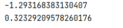
交叉熵的计算：
对应位置按公式计算，即
H = 1* log(0.8) + 1* log(0.7)+ 1* log(0.7)+ 1* log(0.7)

H = 1 * np.log(0.8) + 1 * np.log(0.7) + 1 * np.log(0.7) + 1 * np.log(0.7)
print(H)
h = -H / 4
print(h)

结果如下，最终结果和Tensorflow的结果一致。

• 数据验证阶段，我们发现从二维以后Tensorflow计算的结果和numpy计算的结果不同.
• 上面的验证数据，我们已经对p进行了one-hot编码。
• 如上所述，tensorlfow默认channel_last，即：（batch,hegith,width,channel），默认第一维为batch。
• 将numpy计算的结果除以（batch*height *width）,二者的计算结果会一致。
• Tensorflow中交叉熵函数计算的结果是所有像素点（通道方向上，即“大饼上下对应的点”）的交叉熵和的平均值。

参考文献

[1] https://www.cnblogs.com/wangguchangqing/p/12068084.html
[2] https://blog.csdn.net/tsyccnh/article/details/79163834
[3] https://blog.csdn.net/rtygbwwwerr/article/details/50778098
[4] https://www.khanacademy.org/computing/computer-science/informationtheory/moderninfotheory/v/information-entropy
[5] https://www.youtube.com/watch?v=ErfnhcEV1O8&ab_channel=Aur%C3%A9lienG%C3%A9ron
[6] https://www.zhihu.com/question/41252833
[7] https://www.zhihu.com/question/20994432