深度学习目标跟踪
1. 实质:通过卷积神经网络得到特征图,输出分类和位置。
2. 目标跟踪的分类:
① 单类多目标跟踪:MTCNN、Retinaface…
② 多类多目标跟踪:RCNN、SPP-Net、Fast-RCNN/Faster-RCNN、SSD…
(1) RCNN:
通过聚类得到搜索框(强行缩放),在通过卷积提取特征,最后放入SVM进行分类。
速度慢,准确率不高。
(2) SPP-Net:
主要使用了空间金字塔池化,对不同尺寸的框进行缩放。使得缩放后的尺寸,可以进入FC层,进行输出。
(4)Fast-RCNN:
步骤:CNN卷积、候选框、ROIPooling层、FC输出。
候选框是通过选择性搜索得到,找到所有的候选框十分耗时。
ROIPooling层的目的是将候选框resize到统一的大小。
(5)Faster-RCNN
将FastRCNN中的ROI,替换成RPN网络。
(6)总结:
可见大部分多类多目标的跟踪中,主要问题和改进都集中在对候选框的选择,在yoloV2以后候选框的选择引入了anchor机制。
yolo (you only look once)
1. yoloV1:
(1)步骤:
第一步,先将原图划分为S * S的格子。(7*7)每个格子都有自己的置信度,通过置信度判断格子有无目标,并且进行分类。如果格子有目标,则进入第二步。
第二步,每个格子根据其中心点都可以得到两个建议框,(提前设置以中心点为原点的两个框/实质就是anchor框)即中心点固定,建议框和实际框做偏移。
(2)缺点:一个格子只能确定一种目标。(实际图片中,一个格子包含的信息可能不止一个/种目标);并且当存在小物体或者大物体时,很难预测得到。
(3)输入输出:输入为448 * 448 * 3的图片,输出7 * 7 * (5 * 2 + 20)。即49个格子,每个格子2个anchor框(置信度+坐标位置),20个类别。
(4)损失函数:置信度loss + 坐标loss + 类别loss。
2. yoloV2
(1)主干网络:darknet19
整个网络都是卷积,因此可以多尺寸输入。
实际使用anchor机制将输入改成416 * 416。
输出层则通过一个输出层改为我们所需要的输出。
(2)anchor:根据数据集的真实框位置,通过聚类得到五个anchor框,作为每个格子的建议框。
(3)输入输出:输入为416 * 416 * 3 的图片,输出13 * 13 * 5 * (5 + 20)。即把图片划分成13 * 13个格子,每个格子5个anchor框,每个anchor框都有一个类别标签(20个类别)。
(4) 偏移量:标签都是换算成偏移量进行运算。
预测点中心的位置:cx,cy -> offcx offcy
(例如:实际中心点的位置,cx = 13*(offcx + index),offcx中心点相对于格子左上角的偏移量、 index格子的索引)
即神经网络的输出,每个格子有5个anchor中心,每个中心通过格子大小都可以反算得到实际位置。
预测框的宽高:bw bh ->offw offh
宽高为,预测框与 实际框的比值,在进行log运算(使得偏移量在0附近,防止梯度弥散)。
(4)损失函数:置信度loss + 坐标loss + 类别loss。 区别与yoloV1,这里每个anchor都有自己的类别标签。
3. yolo9000
构建树结构进行分类。具体没详细理解,可以看这个。
4. yoloV3
(1)主干网络:darknet53
主干网络结构中,最后三次下采样得到的特征图都会作为预测。
简单来说,就是不同尺寸的特征图,每个格子代表的感受野不同。下层的感受野比上层更大,含有的语义信息更丰富,因此上层与下层叠加可以保留更多的语义信息。最后进入预测层得到输出。因为最后三次下采样分别预测,(分别是13 * 13、 26 * 26、 52 * 52 大小的特征图)每个格子都有三个anchor框,根据特征图的尺寸不同,预测的物体小大也不同。
详细解读可以看这个
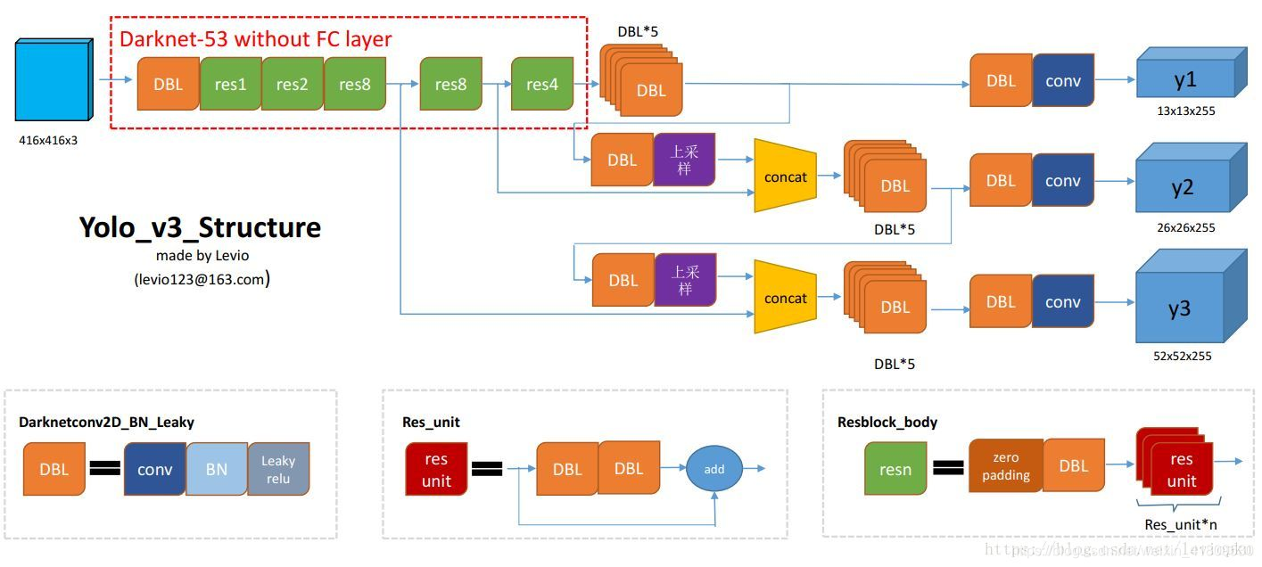
我这里用pytorch自己编写了yoloV3的网络结构,下面是主网络部分,部分网络块得自己编写,例如ConvolutionalLayer为DBL(卷积、batchnorm、relu激活)、下采样块、上采样块、残差网络…
第三次下采样自己作为预测输出,最后第二次下采样输出和第三次下采样得特征图(通过上采样后)做叠加;同理第一次下采样和第二次、第三次叠加后得特征图做叠加。
class yoloV3_net(nn.Module):
    def __init__(self):
        super(yoloV3_net,self).__init__()

        self.trunk_52 = nn.Sequential(
            ConvolutionalLayer(3,32,3,1,1),
            DownsamplingLayer(32,64),
            ResidualLayer(64),
            DownsamplingLayer(64,128),
            ResidualLayer(128),
            ResidualLayer(128),
            DownsamplingLayer(128,256),
            ResidualLayer(256),
            ResidualLayer(256),
            ResidualLayer(256),
            ResidualLayer(256),
            ResidualLayer(256),
            ResidualLayer(256),
            ResidualLayer(256),
            ResidualLayer(256),
        )

        self.trunk_26 = nn.Sequential(
            DownsamplingLayer(256,512),
            ResidualLayer(512),
            ResidualLayer(512),
            ResidualLayer(512),
            ResidualLayer(512),
            ResidualLayer(512),
            ResidualLayer(512),
            ResidualLayer(512),
            ResidualLayer(512),
        )

        self.trunk_13 = nn.Sequential(
            DownsamplingLayer(512,1024),
            ResidualLayer(1024),
            ResidualLayer(1024),
            ResidualLayer(1024),
            ResidualLayer(1024),
        )

        self.convset_13 = nn.Sequential(
            ConvolutionalSet(1024,512)
        )
        self.detetion_13 = nn.Sequential(
            ConvolutionalLayer(512,1024,3,1,1),
            nn.Conv2d(1024,3*(5+5),1,1,0)
        )

        self.up_26 = nn.Sequential(
            ConvolutionalLayer(512,256,1,1,0),
            UpsampleLayer()
        )
        self.convset_26 = nn.Sequential(
            ConvolutionalSet(768,256)
        )
        self.detetion_26 = nn.Sequential(
            ConvolutionalLayer(256, 512, 3, 1, 1),
            nn.Conv2d(512, 3*(5+5), 1, 1, 0)
        )

        self.up_52 = nn.Sequential(
            ConvolutionalLayer(256, 128, 1, 1, 0),
            UpsampleLayer()
        )
        self.convset_52 = nn.Sequential(
            ConvolutionalSet(384, 128)
        )
        self.detetion_52 = nn.Sequential(
            ConvolutionalLayer(128, 256, 3, 1, 1),
            nn.Conv2d(256, 3*(5+5), 1, 1, 0)
        )

    def forward(self,x):
        # 卷积层得到不同尺寸的特征图
        h_52 = self.trunk_52(x)
        h_26 = self.trunk_26(h_52)
        h_13 = self.trunk_13(h_26)
        # 13
        convset_out_13 = self.convset_13(h_13)
        detetion_out_13 = self.detetion_13(convset_out_13)
        up_13to26 = self.up_26(convset_out_13)
        # 26
        route_out_13and26 = torch.cat((up_13to26,h_26),dim=1)
        convset_out_26 = self.convset_26(route_out_13and26)
        detetion_out_26 = self.detetion_26(convset_out_26)
        up_26to52 = self.up_52(convset_out_26)
        # 52
        route_out_26and52 = torch.cat((up_26to52, h_52), dim=1)
        convset_out_52 = self.convset_52(route_out_26and52)
        detetion_out_52 = self.detetion_52(convset_out_52)
        return detetion_out_13,detetion_out_26,detetion_out_52
(2)数据:coco数据集——由于电脑带不动yolo得训练,所以在学习得时候,自己挑选100多张图片,5个类别进行训练。(得到过拟合版本——即训练集为测试集)
① 首先将数据缩放至416 * 416。等比例缩放,缺少部分用黑色填充。
import cv2
import os
def cv2_letterbox_image(image, expected_size):
    ih, iw = image.shape[0:2]
    ew, eh = expected_size,expected_size
    scale = min(eh / ih, ew / iw) # 最大边缩放至416得比例
    nh = int(ih * scale)
    nw = int(iw * scale)
    image = cv2.resize(image, (nw, nh), interpolation=cv2.INTER_CUBIC) # 等比例缩放,使得有一边416
    top = (eh - nh) // 2 # 上部分填充的高度
    bottom = eh - nh - top  # 下部分填充的高度
    left = (ew - nw) // 2 # 左部分填充的距离
    right = ew - nw - left # 右部分填充的距离
    # 边界填充
    new_img = cv2.copyMakeBorder(image, top, bottom, left, right, cv2.BORDER_CONSTANT)
    return new_img

if __name__ == '__main__':
    dir_root = "D:/AIstudyCode/data/yolo_data"
    save_dir = "data/"
    count = 0
    for path in os.listdir(dir_root):
        print(path)
        img = cv2.imread(f"D:/AIstudyCode/data/yolo_data/{path}")
        print(img.shape)
        new_img = cv2_letterbox_image(img,416)
        print(new_img.shape)
        cv2.imwrite(f"{save_dir}images/{count}.jpg",new_img)
        count += 1
        cv2.imshow("1",new_img)
        cv2.waitKey(5)
② 然后通过精灵标注助手进行标注,得到xml标签,进行解析。得到标签文件txt,(便于做dataset)
格式为:文件名path 第一个anchor:类别c (box信息)第二个anchor:类别c (box信息)……

③ dataset:对标签和图片进行解析,并且计算偏移量。
class MyDataset(Dataset):
    def __init__(self):
        with open(LABEL_FILE_PATH) as f:
            self.dataset = f.readlines() # 逐行读取标签文本
            # img_path 类别1 anchor框4 类别1 anchor框4 类别1 anchor框4…
    def __len__(self):
        return len(self.dataset) # 每行代表一个数据 有多少行就有多少数据

    def __getitem__(self, index):
        labels = {

    } # 标签 字典 图片path : 类别
        line = self.dataset[index] # 索引index
        strs = line.split() # 按空格划分每一行
        #_img_data = Image.open(os.path.join(IMG_BASE_DIR,strs[0])) # 路径dir+path
        _img_data = Image.open(os.path.join(strs[0]))

        img_data = transfroms(_img_data) # 数据预处理

        # 将读取得标签 后面类别和置信度从字符格式转换为浮点型 并且用list保存
        #_boxes = np.array(float(x) for x in strs[1:])
        _boxes = np.array(list(map(float,strs[1:])))

        # 例如有三个box  则为 1 *  15(类别1 x1 y1 x2 y2 ……): 转换成 1 * 3 * 5
        boxes = np.split(_boxes, len(_boxes) // 5) # 将anchor分开

        # ANCHORS_GROUP 特征大小(13,26,52):3个anchor的尺寸(w,h)
        for feature_size, anchors in cfg.ANCHORS_GROUP.items():
            # F*F *3*(5+c) 每个格子有三个anchor box c个分类: 置信度1+box位置4+类别数c
            # 初始化标签存储字典为key:list / 且表初始化为零
            labels[feature_size] = np.zeros(shape=(feature_size,feature_size,3,5+cfg.CLASS_NUM))
            for box in boxes:
                cls, cx, cy, w, h = box # 获取标签文本中的真实框

                # modf 分别取出小数部分和整数部分  (实际框的位置等于 特征大小*(索引+偏移量))
                cx_offset, cx_index = math.modf(cx * feature_size / cfg.IMG_WIDTH)
                cy_offset, cy_index = math.modf(cy * feature_size / cfg.IMG_WIDTH)
                # 取出不同特征大小下 提前规定好的anchor尺寸信息
                for i, anchor in enumerate(anchors):
                    # 当前anchor尺寸下的面积
                    anchor_area = cfg.ANCHORS_GROUP_AREA[feature_size][i]
                    # pw ph 实际框和anchor的比值 再取对数 : 网络训练得到_pw,_ph -> 通过 exp(_pw)*anchor_w / exp(_ph)*anchor_h 得到真实框
                    p_w, p_h = w / anchor[0], h / anchor[1]
                    _p_w, _p_h = np.log(p_w),np.log(p_h)
                    #print(_p_h,_p_w)
                    #实际框的面积
                    p_area = w * h
                    # iou取最小框/最大框 : 为了使得iou(充当置信度)小于1大于0 又偏向1
                    iou = min(p_area,anchor_area) / max(p_area, anchor_area)
                    # 对标签存储字典进行幅值
                    # 置信度 中心的偏移x y 宽和高的偏移值(相对于anchor) onehot类别
                    labels[feature_size][int(cy_index), int(cx_index), i] = np.array(
                        [iou,cx_offset,cy_offset,_p_w,_p_h,*one_hot(cfg.CLASS_NUM,int(cls))])
                    #print(cx_offset)
                    #print(feature_size,cy_index,cx_index,i,"________",labels[feature_size][int(cy_index), int(cx_index), i])
                    #print(img_data)
        return labels[13], labels[26], labels[52], img_data
④ 网络搭建。(前面网络结构)
⑤ 损失设计:置信度loss + 坐标loss + 类别loss。
# 损失
def loss_fn(output, target, alpha):

    # torch.nn.BCELoss() 必须得用sigmoid激活
    conf_loss_fn = torch.nn.BCEWithLogitsLoss() # 二分类交叉熵 -> 置信度 自带sigmoid+BCE

    crood_loss_fn = torch.nn.MSELoss() # 平方差 -> box位置
    cls_loss_fn = torch.nn.CrossEntropyLoss() # 交叉熵 -> 类别
    # NLLLOSS log+softmax

    # N C H W -> N H W C
    output = output.permute(0, 2, 3, 1)
    # N C H W -> N H W 3 15
    output = output.reshape(output.size(0), output.size(1), output.size(2), 3, -1)
    output = output.cpu().double()
    mask_obj = target[..., 0] > 0
    output_obj = output[mask_obj]
    target_obj = target[mask_obj]

    loss_obj_conf = conf_loss_fn(output_obj[:,0], target_obj[:,0]) # 置信度损失
    loss_obj_crood = crood_loss_fn(output_obj[:,1:5],target_obj[:,1:5]) # box损失
    # 交叉熵的损失函数 第一个预测出来的标签,且是onehot 第二个参数为真实标签
    label_tags = torch.argmax(target_obj[:,5:], dim=1)
    #print(output_obj[:, 5:].shape, label_tags.shape)
    loss_obj_cls = cls_loss_fn(output_obj[:, 5:], label_tags) # 类别损失

    loss_obj = loss_obj_cls + loss_obj_conf + loss_obj_crood # 总损失

    mask_noobj = target[..., 0] == 0 # anchor中iou为0的数据进行训练 即置信度为0 负样本 只需要训练与真实标签的置信度
    output_noobj = output[mask_noobj]
    target_noobj = target[mask_noobj]
    loss_noobj = conf_loss_fn(output_noobj[:,0], target_noobj[:, 0])
    # 通过权重进行相加 (权重的比例可根据数据集 正负样本比例来设置)
    loss = alpha * loss_obj + (1 - alpha) * loss_noobj

    return loss
⑥ 训练:
if __name__ == '__main__':

    save_path = "data/checkpoints/myyolo.pt" #权重保存的位置
    myDataset = dataset.MyDataset()
    train_loader = DataLoader(myDataset, batch_size=2, shuffle=True)

    device = torch.device("cuda" if torch.cuda.is_available() else "cpu") #是否有cuda
    net = yoloV3_net().to(device)

    if os.path.exists(save_path):
        net.load_state_dict(torch.load(save_path)) #加载权重
    else:
        print("NO Param!")

    net.train()
    opt = torch.optim.Adam(net.parameters())

    epoch = 0
    while(True):
        sum_loss = 0.
        for target_13, target_26, target_52, img_data in train_loader:
            img_data = img_data.to(device)
            output_13, output_26, output_52 = net(img_data)

            loss_13 = loss_fn(output_13, target_13, 0.5)
            loss_26 = loss_fn(output_26, target_26, 0.5)
            loss_52 = loss_fn(output_52, target_52, 0.5)
            loss = loss_13 + loss_26 + loss_52

            opt.zero_grad()
            loss.backward()
            opt.step()
            sum_loss += loss
            print("loss:",loss.item())
        avg_loss = sum_loss / len(train_loader)
        print("epoch:",epoch,"avg_loss:",avg_loss)
        if epoch % 10 == 0:
            torch.save(net.state_dict(),save_path)
            print('save{}'.format(epoch))

        epoch += 1
⑦ 侦测部分:图片进行缩放至416 * 416 然后进入网络,得到输出。
对输出的偏移量进行反算,再通过iou和nms进行筛选。这里的操作和之前MTCNN类似。
class Detector(torch.nn.Module):
    def __init__(self, save_path):
        super(Detector, self).__init__()

        self.net = yoloV3_net().to(device) # 加载网络
        self.net.load_state_dict(torch.load(save_path)) # 加载权重
        self.net.eval() # 标记这里是测试

    def forward(self, input, thresh, anchors):
        # 输入416*416 输出不同尺寸下每个格子的数据 F*F*3*(5+c)
        output_13, output_26, output_52 = self.net(input)

        #print(output_13.shape)
        # 根据置信度筛选boxes 返回索引位置和筛选后的boxes信息
        idxs_13, vecs_13 = self._filter(output_13.to(_device), thresh)
        # 反算box在原照片中的位置
        boxes_13 = self._parse(idxs_13, vecs_13, 32, anchors[13])
        idxs_26, vecs_26 = self._filter(output_26.to(_device), thresh)
        boxes_26 = self._parse(idxs_26, vecs_26, 16, anchors[26])
        idxs_52, vecs_52 = self._filter(output_52.to(_device), thresh)
        boxes_52 = self._parse(idxs_52, vecs_52, 8, anchors[52])
        # 返回最终得到的box信息
        # print(boxes_13.shape)
        # print(boxes_26.shape)
        # print(boxes_52.shape)
        return torch.cat([boxes_13, boxes_26, boxes_52], dim=0)

    def _filter(self, output, thresh):
        output = output.permute(0,2,3,1) # N 3*(5+C) F F -> N F F 3*(5+C)
        output = output.reshape(output.size(0), output.size(1), output.size(2), 3, -1) # N F F 3*(5+C) -> N F F 3 5+C
        #print("1", output[:, 0])
        torch.sigmoid_(output[..., 0])
        #print("2",output[:, 0])

        mask = output[..., 0]>thresh # 5+C = 置信度 + cx cy w h 第0位即为置信度
        #print(output[:, 0])
        idxs = mask.nonzero() # 得到筛选后的位置索引
        #print("idxs",idxs.shape)
        vecs = output[mask] # 得到筛选后的boxes信息
        return idxs, vecs

    def _parse(self, idxs, vecs, t, anchors):
        anchors = torch.Tensor(anchors)
        a = idxs[:,3] # 三个anchor框
        confidence = vecs[:, 0]
        _classify = vecs[:, 5:]
        if len(_classify) == 0:
            classify = torch.Tensor([])
        else:
            classify = torch.argmax(_classify, dim=1).float() # one-hot -> 类别

        # 反算过程
        cy = (idxs[:, 1].float() + vecs[:, 2]) * t
        cx = (idxs[:, 2].float() + vecs[:, 1]) * t
        w = anchors[a, 0] * torch.exp(vecs[:, 3])
        h = anchors[a, 1] * torch.exp(vecs[:, 4])
        x1 = cx - w / 2
        y1 = cy - h / 2
        x2 = x1 + w
        y2 = y1 + h
        out = torch.stack([confidence, x1, y1, x2, y2, classify],dim=1)
        return out
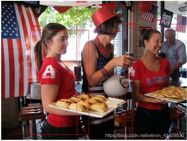
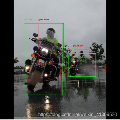
(2)结果:
下面是使用训练的图片作为测试。(电脑配置过低,无法对coco训练集全部训练,所以挑选部分图片,实现过拟合版:仅供学习。。yoloV3的源代码训练过程,是有先用ImageNet数据集对darknet网络做预训练,在迁移到coco数据集上做训练。)具体可以去github下载官方源码和权重包。进行修改和预训练。