Outline
- Light sources.
- Some notes about radiometry.
- Photometric stereo.
- Uncalibrated photometric stereo.
- Generalized bas-relief ambiguity.
Light sources
some useful lighting models
-
plenoptic function (function on 5D domain)
- L ( x , ω ) L(x, \omega) L(x,ω)
-
far-field illumination (function on 2D domain)
- assume that all source of incoming flux are relatively far away
- L ( ω ) L(\omega) L(ω)
-
low-frequency far-field illumination (nine numbers)
- L ( ω ) = ∑ i a i Y i ( ω ) L(\omega)=\sum_i a_i Y_i(\omega) L(ω)=∑iaiYi(ω)
-
directional lighting (three numbers = direction and strength)
-
assumption1: Lambertian
-
assumption2: directional lighting
-
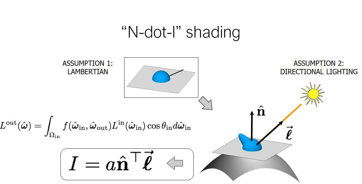
I = a n ^ ⊤ ℓ ⃗ I=a\hat{\bf n}^\top\vec{\boldsymbol{\ell}} I=an^⊤ℓ
- point source (four numbers = location and strength)
Some notes about radiometry
Radiometry vs Photometry
- Radiometry is the field of metrology related to the physical measurement of the properties of electromagnetic radiation, including visible light.
- Photometry describes the effects of visible light on the human eye, in terms of brightness and colour.
Measurement of a sensor using a thin lens
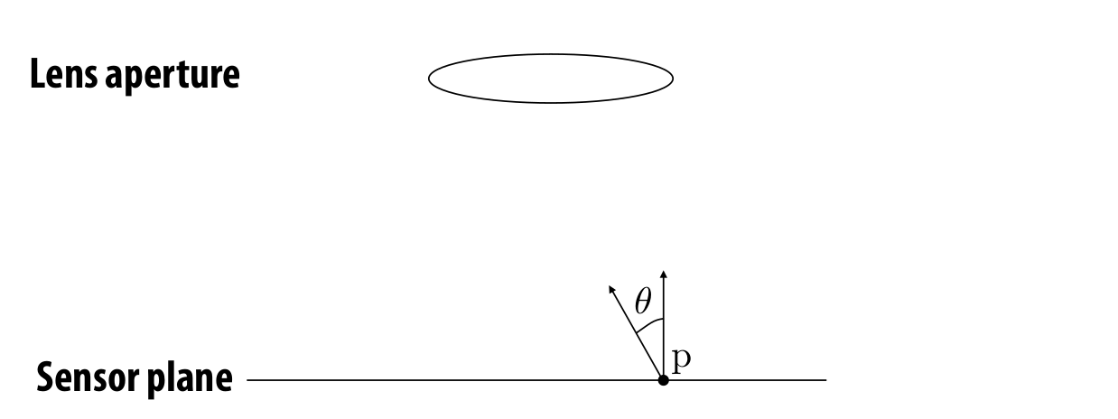
E ( p ) = ∫ hemisphere L i ( p , ω ) cos θ d ω E(p) = \int_{\text{hemisphere}}L_i(p, \omega)\cos\theta d\omega E(p)=∫hemisphereLi(p,ω)cosθdω
transform this integral over the hemisphere to an integral over the aperture area
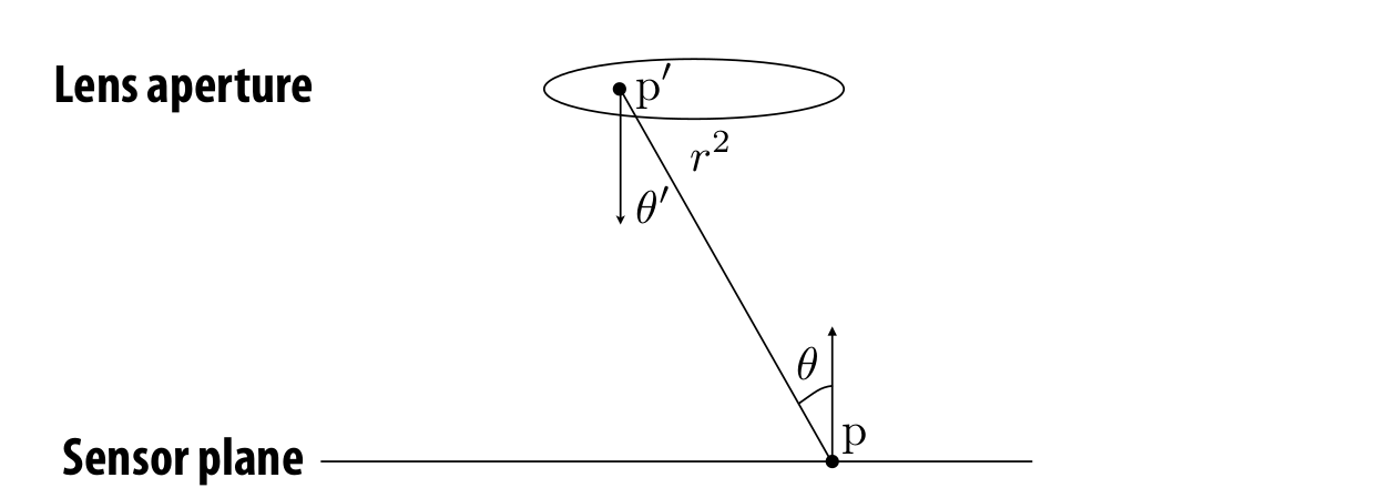
E ( p ) = ∫ aperture L ( p ′ → p ) cos θ cos θ ′ ∥ p ′ − p ∥ 2 d A = sensor are parallel assume aperture and ∫ aperture L ( p ′ → p ) cos 2 θ ∥ p ′ − p ∥ 2 d A = ∥ p − p ′ ∥ = d cos θ 1 d 2 ∫ aperture L ( p ′ → p ) cos 4 θ d A \begin{aligned} E(p) & = \int_{\text{aperture}} L(p'\rightarrow p) \dfrac{\cos\theta\cos\theta'}{\|p'-p\|^2}dA \\ & \xlongequal[\text{sensor are parallel}]{\text{assume aperture and}} \int_{\text{aperture}} L(p'\rightarrow p) \dfrac{\cos^2\theta}{\|p'-p\|^2}dA \\ & \xlongequal{\|p-p'\|=\frac{d}{\cos\theta}} \dfrac{1}{d^2} \int_{\text{aperture}} L(p'\rightarrow p) \cos^4\theta dA \end{aligned} E(p)=∫apertureL(p′→p)∥p′−p∥2cosθcosθ′dAassume aperture andsensor are parallel∫apertureL(p′→p)∥p′−p∥2cos2θdA∥p−p′∥=cosθdd21∫apertureL(p′→p)cos4θdA
which means that pixels far off the center receive less light

BTW: Four types of vignetting
- Mechanical: light rays blocked by hoods, filters, and other objects.
- Lens: similar, but light rays blocked by lens elements.
- Natural: due to radiometric laws (“cosine fourth falloff”).
- Pixel: angle-dependent sensitivity of photodiodes.

Photometric stereo
Outline
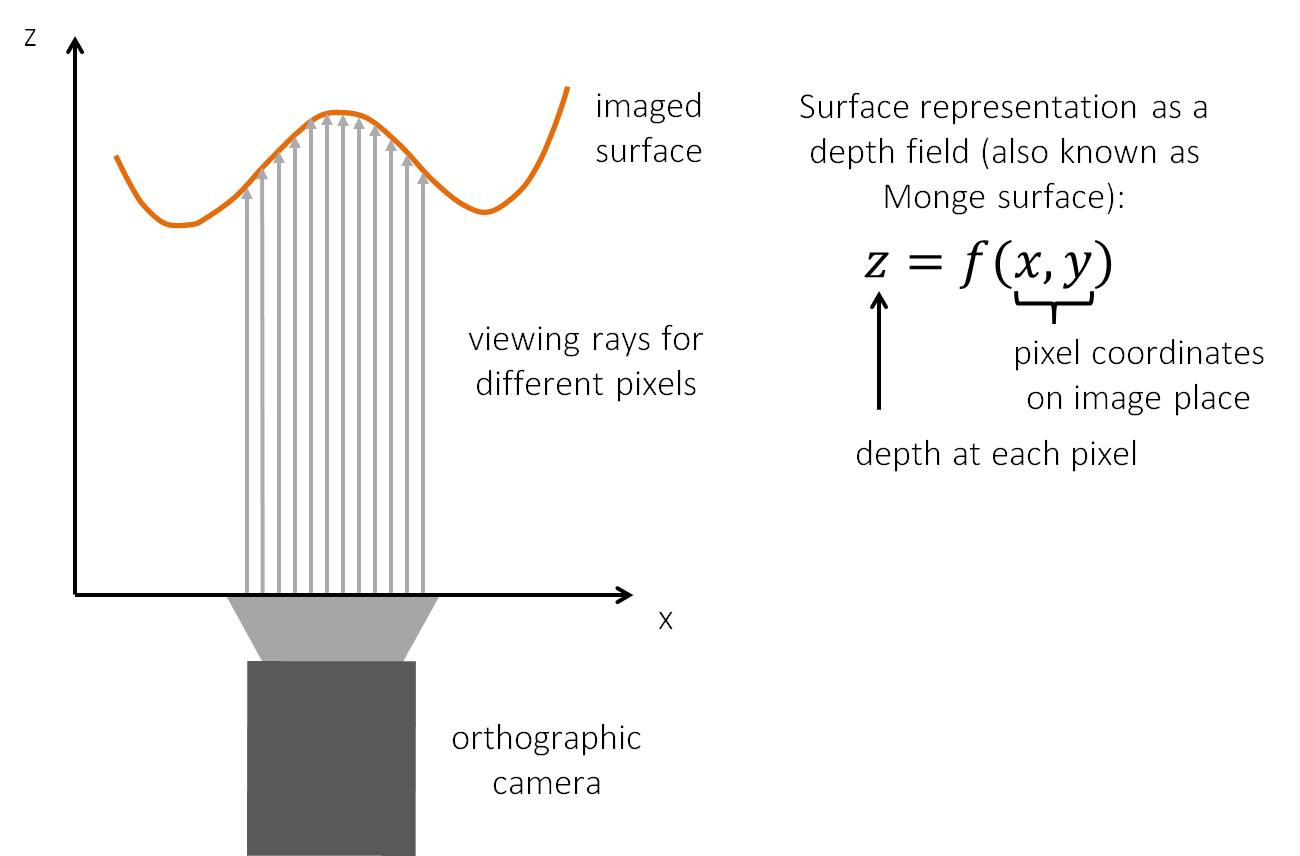
- 用orthographic camera测定 I I I
- 用chrome sphere测定光源方向 ℓ ⃗ \vec{\boldsymbol{\ell}} ℓ
- 由 I = a n ^ ⊤ ℓ ⃗ I=a\hat{\bf n}^\top\vec{\boldsymbol{\ell}} I=an^⊤ℓ 解出 n ^ \hat n n^
- 把 n ^ \hat n n^ 积分得到depth
1 用orthographic camera测定 I I I
2 用chrome sphere测定光源方向 ℓ ⃗ \vec{\boldsymbol{\ell}} ℓ
there are limitations: see P67
3 由 I = a n ^ ⊤ ℓ ⃗ I=a\hat{\bf n}^\top\vec{\boldsymbol{\ell}} I=an^⊤ℓ 解出 n ^ \hat n n^
注意以下讨论的前提是directional lighting模型,即假设朗伯面+单向光源

I 1 = a n ^ ⊤ ℓ ⃗ 1 b ⃗ ≜ a n ^ [ I 1 I 2 ⋮ I N ] N × 1 = [ ℓ ⃗ 1 ⊤ ℓ ⃗ 2 ⊤ ⋮ ℓ ⃗ N ⊤ ] N × 3 [ b ⃗ ] 3 × 1 I_1=a\hat{\boldsymbol{n}}^\top\vec{\boldsymbol{\ell}}_1 \\ \vec{\boldsymbol{b}}\triangleq a\hat{\boldsymbol{n}} \\ \left[\begin{array}{c} I_1 \\ I_2 \\ \vdots \\ I_N \end{array}\right]_{N\times 1}\!\!\!\!\! =\left[\begin{array}{c} \vec{\boldsymbol{\ell}}_1^\top \\ \vec{\boldsymbol{\ell}}_2^\top \\ \vdots \\ \vec{\boldsymbol{\ell}}_N^\top \\ \end{array}\right]_{N\times 3}\!\!\!\!\!\!\!\!\! \left[\begin{array}{c} \vec{\boldsymbol{b}} \end{array}\right]_{3\times 1} I1=an^⊤ℓ1b≜an^⎣⎢⎢⎢⎡I1I2⋮IN⎦⎥⎥⎥⎤N×1=⎣⎢⎢⎢⎢⎢⎡ℓ1⊤ℓ2⊤⋮ℓN⊤⎦⎥⎥⎥⎥⎥⎤N×3[b]3×1
b ⃗ \vec{\boldsymbol{b}} b 是三维的,因此理论上 N ≥ 3 N \ge 3 N≥3 才能解出 b ⃗ \vec{\boldsymbol{b}} b 而不损失信息
实际上解总有误差,因此 N N N 越大越好,我们求解一下方程的最小均方解
I = L b ⃗ I = L\vec{\boldsymbol{b}} I=Lb
解可用伪逆表示
b ⃗ = L + I \vec{\boldsymbol{b}} = L^+I b=L+I
4 把 n ^ \hat n n^ 积分得到depth
Use vector field integration techniques as in gradient-domain image processing.
Uncalibrated photometric stereo
如果不知道光源信息,这时候又该怎么恢复depth?
考虑图片中的所有像素,设共有 M M M 个
[ I 1 I 2 ⋮ I N ] N × M = [ ℓ ⃗ 1 ⊤ ℓ ⃗ 2 ⊤ ⋮ ℓ ⃗ N ⊤ ] N × 3 [ B ] 3 × M \left[\begin{array}{c} I_1 \\ I_2 \\ \vdots \\ I_N \end{array}\right]_{N\times M}\!\!\!\!\! =\left[\begin{array}{c} \vec{\boldsymbol{\ell}}_1^\top \\ \vec{\boldsymbol{\ell}}_2^\top \\ \vdots \\ \vec{\boldsymbol{\ell}}_N^\top \\ \end{array}\right]_{N\times 3}\!\!\!\!\!\!\!\!\! \left[\begin{array}{c} B \end{array}\right]_{3\times M} ⎣⎢⎢⎢⎡I1I2⋮IN⎦⎥⎥⎥⎤N×M=⎣⎢⎢⎢⎢⎢⎡ℓ1⊤ℓ2⊤⋮ℓN⊤⎦⎥⎥⎥⎥⎥⎤N×3[B]3×M
简记为
I N × M = L N × 3 B 3 × M I_{N\times M} = L_{N\times3}B_{3\times M} IN×M=LN×3B3×M
排除种种近似和测量误差,理论上 r a n k ( I ) = 3 rank(I)=3 rank(I)=3,因此我们要找 I I I 的一个low-rank approximation。怎么找?对 I I I 进行SVD分解,只保留前三个分量即可。
通过SVD分解,我们也找到了 L L L 和 B B B 的表示,可惜这种表示不唯一,对于任意可逆矩阵 Q 3 × 3 Q_{3\times3} Q3×3, L Q − 1 LQ^{-1} LQ−1 和 Q B QB QB 也是可行解。
目前的不确定性完全由矩阵 Q Q Q 来衡量,自由度为9,有什么办法能降低一些自由度?
Generalized bas-relief ambiguity
注意到surface是光滑的(就算不光滑也是可以忽略不计的局部),这就要求法向量们 N N N 必须是可积的。
然而这还不够,只能降低自由度到3。具体的数学原理有待进一步学习。
不过物体的形状已经八九不离十了,唯一不确定的就是如何抻拉的问题?
reference:
CMU 15-463: lecture 18