特征选择三种方法:
-
Filter(过滤法)
-
Wrapper(包装法)
-
Embedded(嵌入法)
过滤法
卡方检验
直接看sklearn代码:
首先做OHE
Y = LabelBinarizer().fit_transform(y)
做完之后 Y Y Y的shape是 N × K N\times K N×K
observed = safe_sparse_dot(Y.T, X) # n_classes * n_features
K , N × N , M K,N\times N,M K,N×N,M
形成一个 K × M K\times M K×M的矩阵,表示每个类别对应的特征之和
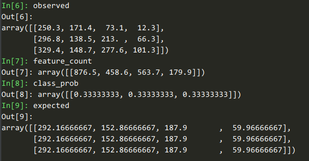
observed
Out[6]:
array([[250.3, 171.4,  73.1,  12.3],
       [296.8, 138.5, 213. ,  66.3],
       [329.4, 148.7, 277.6, 101.3]])
最后算卡方的代码:
def _chisquare(f_obs, f_exp):
    """Fast replacement for scipy.stats.chisquare.

    Version from https://github.com/scipy/scipy/pull/2525 with additional
    optimizations.
    """
    f_obs = np.asarray(f_obs, dtype=np.float64)

    k = len(f_obs)
    # Reuse f_obs for chi-squared statistics
    chisq = f_obs
    chisq -= f_exp
    chisq **= 2
    with np.errstate(invalid="ignore"):
        chisq /= f_exp
    chisq = chisq.sum(axis=0)
    return chisq, special.chdtrc(k - 1, chisq)
自变量对因变量的相关性
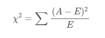
A A A是观测, E E E是期望, 其shape都是 K × M K\times M K×M
自变量有 N N N种取值,因变量有 M M M种取值,考虑自变量等于 i i i且因变量等于 j j j的样本频数的观察值与期望的差距,构建统计量