文章目录
作业介绍
题目要求:二元分类是机器学习中最基础的问题之一,在这份教学中,你将学会如何实现一个线性二元分类器,来根据人们的个人资料,判断其年收入是否高于 50,000 美元。我们将用两种方法**logistic regression 与 generative model **来达成以上目的(另文章有点长,会将第二种方法放在另一篇博文里)。
所需的数据资料点击此链接免费下载 https://download.csdn.net/download/qq_46126258/14926677
在训练过程中,只有 X_train、Y_train 和 X_test 这三个资料经过处理的文件会被经常使用到,train.csv 和 test.csv 这两个原始资料则可以提供你一些额外的信息。
其中打开原始资料train.csv后发现可以用age、class of worker、detailed industry recode、education、wage per hour、enroll in edu inst last wk、marital stat、major industry code、major occupation code、race、hispanic origin、sex、member of a labor union、reason for unemployment、full or part time employment stat、capital gains、capital losses等 ( 41 列 ) \color{red}(41列) (41列)的特征来描述并判断他的工资情况。
为了进一步数值化的表示,在X_train中则对train.csv中非数字的部分通过扩展特征名称使其可以用数字表示。如:train.csv中的在哪里工作,有在学校、在公司等等答案,在X_train则用是否在学校工作、是否在公司工作来代替表示。类似地扩展后我们在X_train得到了一行特别长的特征 ( 510 列 ) \color{red}(510列) (510列)来描述一个人的工资情况。
一、logistic regression
提示:
训练集(training set):包括X_train + Y_train
验证集(development set/ validation set):包括X_dev + Y_dev
测试集(testing set):包括X_test
我们通过训练集的X_train + Y_train训练估计参数,在验证集上求取准确率,在测试集上进行预测,并保存答案到文件。
1、Preparing data
(1)载入数据
手动打开X_train,查看数据形式:第一行是特征的名称,我们需要从第二行开始截取。按行读取信息从下标为1的列开始(跳过id那一列)

手动打开Y_train,查看数据形式:按行读取,跳过第一行,只截取第1列(下标为1)
由于要打开三个文件X_train、Y_train 和 X_test,我们引入一种类似C语言的文件打开方式,具体补充详见链接https://www.cnblogs.com/ymjyqsx/p/6554817.html
补 充 知 识 点 : \color{red}补充知识点: 补充知识点:
line.strip(’\n’).split(’,’)
strip(’\n’)表示删除掉数据中的换行符,split(‘,’)则是数据中遇到‘,’ 就隔开。
import numpy as np

np.random.seed(0) #当我们设置相同的seed,每次生成的随机数相同
X_train_fpath = './data/X_train'
Y_train_fpath = './data/Y_train'
X_test_fpath = './data/X_test'
output_fpath = './output_{}.csv'#接收结果

with open(X_train_fpath) as f:
    next(f) #跳过第一行,从第二行开始读取
    #截取每行下标为1到最后的列,删除掉每行数据中的换行符,遇到','分割数据
    X_train = np.array([line.strip('\n').split(',')[1:] for line in f],dtype=float)

with open(Y_train_fpath) as f:
    next(f)
    Y_train = np.array([line.strip('\n').split(',')[1] for line in f],dtype=float )

with open(X_test_fpath) as f:
    next(f)
    X_test = np.array([line.strip('\n').split(',')[1:] for line in f],dtype=float)
(2)定义能求某特定列均值和方差,并根据此值对矩阵X做正则化的函数
X:待处理的矩阵,处理后作为返回值
train:为‘True’表示处理的是training data,‘False’表示处理的是testing data
specified_column:一个数,表示某列,如果不为’None’,返回一个数;如果为‘none’表示求取所有列的均值和方差,返回1×n的矩阵
X_mean ,X_std:事先定义并作为结果的返回值
之所以要设置train这一参数,是因为对X_test进行正则化化的时候实际上应该用训练集X_train的均值和方差。因此train为‘True’计算训练集的均值方差,为‘False’时,在传递参数时使用之前得到均值方差
def _normalize(X, train = True, specified_column = None, X_mean = None, X_std = None):
    '''
    This function normalizes specific columns of X.
    The mean and standard variance of training data will be reused when processing testing data.

    :param X: data to be processed
    :param train: 'True' when processing training data,'False' for tseting data
    :param specified_column: indexs of the columns that will be normalized.
                              if 'none' all collumn will be normalized.
    :param X_mean: mean value of training data,used when train = 'False'
    :param X_std: standard deviation of training data, used when train = 'False'

    :return:
    X: normalized data
    X_mean:computed mean value of training data
    X_std:computed standard deviation of training data
    '''

    if specified_column == None:
        specified_column = np.arange(X.shape[1])
    if train:
        X_mean = np.mean(X[:,specified_column], 0).reshape(1,-1)
        X_std = np.std(X[:,specified_column], 0).reshape(1,-1)

    X[:,specified_column] = (X[:, specified_column] - X_mean) / (X_std + 1e-8)
    #+ 1e-8防止分母为0

    return X, X_mean, X_std
补 充 知 识 点 : \color{red}补充知识点: 补充知识点:
np.mean(matrix,axis=0) 其中 matrix为一个矩阵,axis为参数
以 m×n 矩阵举例:
axis 不设置值,对 m*n 个数求均值,返回一个实数
axis = 0:压缩行,对各列求均值,返回 1×n 矩阵
对X_train,X_test进行正则化
利用X_train经过_normalize(X_train, train = True)得到每一列的 X_mean, X_std(一个行矩阵),并根据此值对X_test进行正则化。
X_train, X_mean, X_std = _normalize(X_train, train = True)
X_test, _, _ = _normalize(X_test, train=False, specified_column=None,X_mean=X_mean,X_std=X_std)
(3)定义“划分训练集(training set):X_train + Y_train 和验证集(development set/ validation set)X_dev + Y_dev”的函数
dev_ratio = 0.25:表示验证集占0.25;那么测试集:验证集 = 0.75:0.25
返回值:X_train,Y_train,X_dev,Y_dev
def _train_dev_split(X, Y,dev_ratio = 0.25):
    train_size = int(len(X) * (1 - dev_ratio))
    return X[:train_size],Y[:train_size],X[train_size:],Y[train_size:]
从X_train中按照9:1划分训练集和验证集;dev_ratio = 0.1

dev_ratio = 0.1
X_train, Y_train, X_dev, Y_dev = _train_dev_split(X_train, Y_train, dev_ratio=dev_ratio)
(4)求出一些有用的维度数
train_size = X_train.shape[0]
dev_size = X_dev.shape[0]
test_size = X_test.shape[0]
data_dim = X_train.shape[1]
print('Size of training set: {}'.format(train_size))
print('Size of development set: {}'.format(dev_size))
print('Size of testing set: {}'.format(test_size))
print('Dimension of data: {}'.format(data_dim))

'''
Size of training set: 48830
Size of development set: 5426
Size of testing set: 27622
Dimension of data: 510
'''
2、Some Useful Functions
(1)打乱行顺序的函数:
补 充 知 识 点 : \color{red}补充知识点: 补充知识点:
多维矩阵中,只对第一维(行)做打乱顺序操作。也就是每一行的数据不动,但是行的顺序改变。
例:
在一维中,np.random.shuffle(randomize) 将列表randomize内元素打乱顺序
在二维中,randomize记录X的行下标:randomize = np.arange(len(X)),在经过np.random.shuffle(arandomize) 后元素顺序改变;由于randomize与X的下标绑定,randomize内元素顺序改变,那么X的下标也进行同步的改变
def _shuffle(X, Y):
 # This function shuffles two equal-length list/array, X and Y, together.
    randomize = np.arange(len(X))
    np.random.shuffle(randomize)
    return (X[randomize], Y[randomize])
(2)定义sigmoid函数
补 充 知 识 点 : \color{red}补充知识点: 补充知识点:
np.clip(a, a_min, a_max, out=None):
取a数组中的闭区间[a_min, a_max],数组中小于a_min的数都变成a_min,大于a_max的数都变成a_max
如:
a = np.arange(10)
np.clip(a, 1, 8)
array([0, 1, 2, 3, 4, 5, 6, 7, 8, 9]) 会变成 array([1, 1, 2, 3, 4, 5, 6, 7, 8, 8])
使用 np.clip()是为了防止overflow,剔除小于/大于规定的最小值/最大值的数,使经过sigmoid过的数只能在(1e-8)和( 1 - (1e-8) )之间即符合函数特性:两边无限趋近于0/无限趋近于1
def _sigmoid(z):
    # Sigmoid function can be used to calculate probability.
    # To avoid overflow, minimum/maximum output value is set.
    return np.clip(1 / (1.0 + np.exp(-z)), 1e-8, 1 - (1e-8))
(4)定义f(x)函数
np.matmul(X, w)表示矩阵相乘,具体乘法和广播机制的应用请参考链接https://blog.csdn.net/alwaysyxl/article/details/83050137
def _f(X, w, b):
    '''
    This is the logistic regression function, parameterized by w and b

    :param X: input data, shape = [batch_size, data_dimension]
    :param w: weight vector, shape = [data_dimension, ]
    :param b: bias, scalar
    :return: predicted probability of each row of X being positively labeled, shape = [batch_size, ]
    '''
    return _sigmoid(np.matmul(X, w) + b)
(5)对预测结果取整数
补 充 知 识 点 : \color{red}补充知识点: 补充知识点:
np.round(数据, decimal=保留的小数位数)
原则:
一般该函数遵循四舍五入原则:np.round(11.5)=12
但是会有特殊情况:当整数部分以0结束时,一律是向下取整:np.round(10.5)=10
比较稳定的浮点数取整:向上的np.ceil(11.5)=12,向下的floor(11.5)=11
这里我也不太懂为什么要取整数,有大佬可以帮忙解释下哈,感谢
def _predict(X, w, b):
# This function returns a truth value prediction for each row of X
# by rounding the result of logistic regression function.
    return np.round(_f(X, w, b)).astype(np.int)
(6)计算预测准确率
补 充 知 识 点 : \color{red}补充知识点: 补充知识点:
np.abs(x)、np.fabs(x) : 计算数组各元素的绝对值
def _accuracy(Y_pred, Y_label):
    # This function calculates prediction accuracy
    acc = 1 - np.mean(np.abs(Y_pred - Y_label))
    return acc
3、Functions about gradient and loss
(1)定义loss函数即交叉熵

按照公式直接打出来:
def _cross_entropy_loss(y_pred, Y_label):
    '''
    This function computes the cross entropy.

    :param y_pred: probabilistic predictions, float vector
    :param Y_label: ground truth labels, bool vector
    :return: cross entropy, scalar
    '''
    cross_entropy = -np.dot(Y_label, np.log(y_pred)) - np.dot((1 - Y_label), np.log(1 - y_pred))
    return cross_entropy
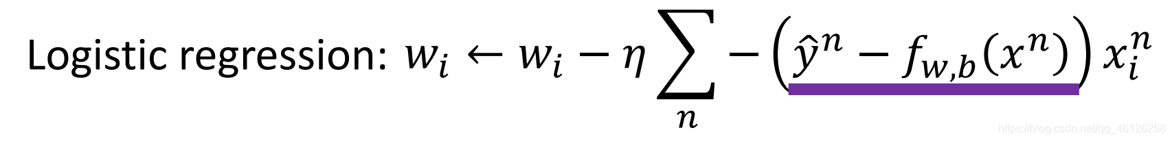
(2)定义gradient函数
loss函数的值最小时对应的 w ∗ , b ∗ w^*,b^* w∗,b∗是最终的估计值,在此之前我们会计算多个loss值并进行比较。在这里的gradient函数只是针对一次梯度下降进行的计算,w的更新方式如下:
def _gradient(X, Y_label, w, b):
    # This function computes the gradient of cross entropy loss with respect to weight w and bias b.
    y_pred = _f(X, w, b)
    pred_error = Y_label - y_pred
    w_grad = -np.sum(pred_error * X.T, 1)
    b_grad = -np.sum(pred_error)
    return w_grad, b_grad
4、Training
我们使用小批次梯度下降法来训练。训练资料被分为许多小批次,针对每一个小批次,我们分别计算其梯度以及损失,并根据该批次来更新模型的参数。当一次循环完成,也就是整个训练集的所有小批次都被使用过后,我们将所有的训练资料打散并重新分为新的小批次,进行下一次循环,直至事先设定的循环次数达成位置。
(1)初始化w、b等参数
w = np.zeros([data_dim, ]) #等价于w = np.zeros((data_dim,))
#data_dim = X_train.shape[1]列数
b = np.zeros([1, ])

max_iter = 10
batch_size =8
learning_rate = 0.2
(2)保存每次迭代时的loss和accuracy用于画图
# Keep the loss and accuracy at every iteration for plotting
train_loss = [] #训练集的loss值
dev_loss = [] #验证集的loss
train_acc = [] #训练集的准确率
dev_acc = [] #验证集的准确率
(3)迭代训练
将 X_train, Y_train 打乱行序后,进行内部分组训练train_size=48830(X_train的行数),每组8行,共train_size/batch_size≈6103组(np.floor向下取整)。
补 充 知 识 点 : \color{red}补充知识点: 补充知识点:
train_acc.append(_accuracy(Y_train_pred, Y_train))中的 .append 表示在列表后面添加值
# Calcuate the number of parameter updates
step = 1

# Iterative training
for epoch in range(max_iter):
    # Random shuffle at the begging of each epoch
    X_train, Y_train = _shuffle(X_train, Y_train)

    # Mini-batch training
    for idx in range(int(np.floor(train_size / batch_size))):
        # 共计6103组,取出每组的X,Y
        X = X_train[idx*batch_size:(idx+1)*batch_size]
        Y = Y_train[idx*batch_size:(idx+1)*batch_size]

        # Compute the gradient
        w_grad, b_grad = _gradient(X, Y, w, b)

        # gradient descent update
        # learning rate decay with time
        w = w - learning_rate/np.sqrt(step) * w_grad
        b = b - learning_rate/np.sqrt(step) * b_grad

        step = step + 1

    # Compute loss and accuracy of training set and development set
    y_train_pred = _f(X_train, w, b)
    Y_train_pred = np.round(y_train_pred) #四舍五入
    train_acc.append(_accuracy(Y_train_pred, Y_train))
    train_loss.append(_cross_entropy_loss(y_train_pred, Y_train) / train_size)

    y_dev_pred = _f(X_dev, w, b)
    Y_dev_pred = np.round(y_dev_pred)
    dev_acc.append(_accuracy(Y_dev_pred, Y_dev))
    dev_loss.append(_cross_entropy_loss(y_dev_pred, Y_dev) / dev_size)
print('Training loss: {}'.format(train_loss[-1]))
print('Development loss: {}'.format(dev_loss[-1]))
print('Training accuracy: {}'.format(train_acc[-1]))
print('Development accuracy: {}'.format(dev_acc[-1]))
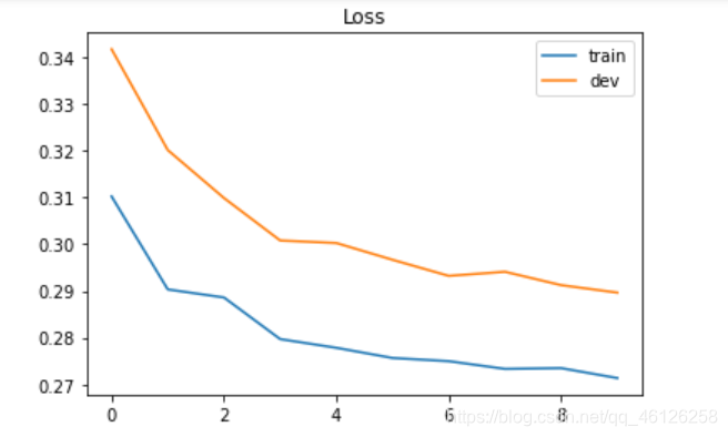
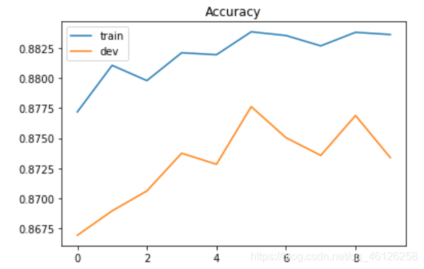
'''
Training loss: 0.27375099679341935
Development loss: 0.29846020164908743
Training accuracy: 0.8825107515871391
Development accuracy: 0.877441946185035
'''
5、Plotting Loss and accuracy curve
画出loss随迭代次数、accuracy随迭代次数的曲线图
import matplotlib.pyplot as plt

# Loss curve
plt.plot(train_loss)
plt.plot(dev_loss)
plt.title('Loss')
plt.legend(['train', 'dev'])
plt.savefig('loss.png')
plt.show()

# Accuracy curve
plt.plot(train_acc)
plt.plot(dev_acc)
plt.title('Accuracy')
plt.legend(['train', 'dev'])
plt.savefig('acc.png')
plt.show()
6、Predicting testing labels
利用求出的w,b预测测试集X_test的结果,并将答案保存在output_logistic.csv中。首先确认上交文件的格式,打开sample_submission.csv有id label两列。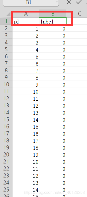
补 充 知 识 点 : \color{red}补充知识点: 补充知识点:
enumerate(predictions) 可以既遍历出predictions的索引,又遍历出元素
# Predict testing labels
predictions = _predict(X_test, w, b)
with open(output_fpath.format('logistic'), 'w') as f:
    f.write('id,label\n')
    for i, label in  enumerate(predictions):
        f.write('{},{}\n'.format(i, label))
我们也可以查看影响一个人工资是否达到 50,000美金的最主要的前10个因素是什么,也就是最大权重
补 充 知 识 点 : \color{red}补充知识点: 补充知识点:
np.argsort(a, axis=-1, kind=‘quicksort’, order=None): 输出x中元素从小到大排列的对应的index(索引)
使用 “kind” 关键字指定的算法,沿给定轴,执行间接排序。它返回一个按给定轴排序的 索引数组 ,该数组与 “a” 形状一样,默认为 -1 (最后一个轴)
np.argsort()[::-1] 输出x中元素从大到小排列的对应的index(索引)
更多用法详见链接
打印w,发现权重有正有负,影响最大的权重应该是根据绝对值进行比较的,所以对w取绝对值再进行排序,再将w从小到大排序的下标数组存入ind:ind = np.argsort(np.abs(w))[::-1],此时各个数值没有相应的keys,所以看不出来最大数对应哪一个特征,我们要将X_train的表头那一行读出来存入features中。根据ind存储的排序下标找到对应的最大features[i],w[i],输出结果就能看出影响的最大比重的是什么了!

# Print out the most significant weights最大的权重
ind = np.argsort(np.abs(w))[::-1] #从小到大排序
with open(X_test_fpath) as f:#读出表头,即对应权重的keys
    content = f.readline().strip('\n').split(',')
features = np.array(content) #将特征列为数组
for i in ind[0:10]:
    print(features[i], w[i])

'''
 Not in universe -4.031960278019252
 Spouse of householder -1.6254039587051399
 Other Rel <18 never married RP of subfamily -1.4195759775765402
 Child 18+ ever marr Not in a subfamily -1.295857207666473
 Unemployed full-time 1.1712558285885906
 Other Rel <18 ever marr RP of subfamily -1.1677918072962366
 Italy -1.093458143800618
 Vietnam -1.0630365633146412
num persons worked for employer 0.9389922773566489
 1 0.8226614922117187
 '''