Heapsort (堆排序)是最经典的排序算法之一,在google或者百度中搜一下可以搜到很多非常详细的解析。同样好的排序算法还有quicksort(快速排序)和merge sort(归并排序),选择对这个算法进行分析主要是因为它用到了一个非常有意思的算法技巧:数据结构 - 堆。而且堆排其实是一个看起来复杂其实并不复杂的排序算法,个人认为heapsort在机器学习中也有重要作用。这里重新详解下关于Heapsort的方方面面,也是为了自己巩固一下这方面知识,有可能和其他的文章有不同的入手点,如有错误,还请指出。文中引用的referecne会再结尾标注。
p.s. 个人认为所谓详解是你在看相关wiki或者算法书看不懂的时候看通俗易懂的解释,不过最佳方案还是去看教授们的讲解,推荐reference[1]中的heapsort章节。
以上是废话,可以不看
Section 1 - 简介
Heapsort是一个comparison-based的排序算法(快排,归并,插入都是;counting sort不是),也是一种选择排序算法(selection sort),一个选择算法(selection algorithm)的定义是找到一个序列的k-th order statistic(统计学中的术语),直白的说就是找到一个list中第k-th小的元素。以上都可以大不用懂,heapsort都理解了回来看一下是这回事就是了。同样,插值排序也是一种选择排序算法。
Heapsort的时间复杂度在worst-case是 O(nlgn) ,average-case是 O(nlgn) ;空间复杂度在worst-case是 O(1) ,也就是说heapsort可以in-place实现;heapsort不稳定。
以下顺便附上几种排序算法的时间复杂度比较( Θ−notation 比 O−notation 更准确的定义了渐进分析(asymptotic analysis)的上下界限,详细了解可以自行google):
| Algorithm | Worst-case |
Average-case/expected |
| Insertion sort(插值排序) |
Θ(n2) | Θ(n2) |
| Merge sort(归并排序) |
Θ(nlgn) | Θ(nlgn) |
| Heapsort(堆排序) | O(nlgn) | O(nlgn) |
| Quicksort(快速排序) | Θ(n2) | Θ(n2) (expected) |
*Additional Part - KNN
heapsort在实践中的表现经常不如quicksort(尽管quicksort最差表现为 Θ(n2) ,但quicksort 99%情况下的runtime complexity为 Θ(nlgn) ),但heapsort的 O(nlgn) 的上限以及固定的空间使用经常被运作在嵌入式系统。在搜索或机器学习中经常也有重要的作用,它可以只返回k个排序需要的值而不管其他元素的值。例如KNN(K-nearest-neighbour)中只需返回K个最小值即可满足需求而并不用对全局进行排序。当然,也可以使用divide-and-conquer的思想找最大/小的K个值,这是一个题外话,以后有机会做一个专题比较下。
以下程序为一个简单的在python中调用heapq进行heapsort取得k个最小值,可以大概体现上面所述的特性:
'''
Created On 15-09-2014

@author: Jetpie

'''


import heapq, time
import scipy.spatial.distance as spd
import numpy as np

pool_size = 100000

#generate an 3-d random array of size 10,000
# data = np.array([[2,3,2],[3,2,1],[2,1,3],[2,3,2]])
data = np.random.random_sample((pool_size,3))
#generate a random input
input = np.random.random_sample()
#calculate the distance list
dist_list =  [spd.euclidean(input,datum) for datum in data]

#find k nearest neighbours
k = 10

#use heapsort
start = time.time()
heap_sorted = heapq.nsmallest(k, range(len(dist_list)), key = lambda x: dist_list[x])
print('Elasped time for heapsort to return %s smallest: %s'%(k,(time.time() - start)))

#find k nearest neighbours
k = 10000

#use heapsort
start = time.time()
heap_sorted = heapq.nsmallest(k, range(len(dist_list)), key = lambda x: dist_list[x])
print('Elasped time for heapsort to return %s smallest: %s'%(k,(time.time() - start)))

get_k_smallest
运行结果为:
Elasped time for heapsort to return 10 smallest: 0.0350000858307
Elasped time for heapsort to return 10000 smallest: 0.0899999141693
Section 2 - 算法过程理解
2.1 二叉堆


在“堆排序”中的“堆”通常指“二叉堆(binary heap)”,许多不正规的说法说“二叉堆”其实就是一个完全二叉树(complete binary tree),这个说法正确但不准确。但在这基础上理解“二叉堆”就非常的容易了,二叉堆主要满足以下两项属性(properties):
#1 - Shape Property: 它是一个完全二叉树。
#2 - Heap Property: 主要分为max-heap property和min-heap property(这就是我以前说过的术语,很重要)
|--max-heap property :对于所有除了根节点(root)的节点 i, A[Parent]≥A[i]
|--min-heap property :对于所有除了根节点(root)的节点 i, A[Parent]≤A[i]
上图中的两个二叉树结构均是完全二叉树,但右边的才是满足max-heap property的二叉堆。
在以下的描述中,为了方便,我们还是用堆来说heapsort中用到的二叉堆。
2.2 一个初步的构想
有了这样一个看似简单的结构,我们可以产生以下初步构想来对数组A做排序:
1.将A构建成一个最大堆(符合max-heap property,也就是根节点最大);
2.取出根节点(how?);
3.将剩下的数组元素在建成一个最大二叉堆,返回第2步,直到所有元素都被取光。
如果已经想到了以上这些,那么就差不多把heapsort完成了,剩下的就是怎么术语以及有逻辑、程序化的表达这个算法了。
2.3 有逻辑、程序化的表达
通常,heapsort使用的是最大堆(max-heap)。给一个数组A(我们使用 Java序列[0...n]),我们按顺序将它初始化成一个堆:
Input: 
Initialization: 
*堆的根节点(root)为A[0];
对这个堆中index为 i 的节点,我们可以得到它的parent, left child and right child,有以下操作:
Parent(i): parent(i)←A[floor((i−1)/2)]
Left(i): left(i)←A[2∗i+1]
Right(i): right(i)←A[2∗i+2]
通过以上操作,我们可以在任意index- i 得到与其相关的其他节点(parent/child)。
在heapsort中,还有三个非常重要的基础操作(basic procedures):
Max-Heapify(A , i): 维持堆的#2 - Heap Property,别忘了在heapsort中我们指的是max-heap property(min-heap property通常是用来实现priority heap的,我们稍后提及)。
Build-Max-Heap(A): 顾名思义,构建一个最大堆(max-heap)。
Heapsort(A): 在Build-Max-Heap(A)的基础上实现我们2.2构想中得第2-3步。
其实这三个操作每一个都是后面操作的一部分。
下面我们对这三个非常关键的步骤进行详细的解释。
Max-Heapify(A , i)
+Max-Heapify的输入是当前的堆A和index- i ,在实际的in-place实现中,往往需要一个heapsize也就是当前在堆中的元素个数。
+Max-Heapify有一个重要的假设:以Left( i )和Right( i )为根节点的subtree都是最大堆(如果树的知识很好这里就很好理解了,但为什么这么假设呢?在Build-Max-Heap的部分会解释)。
+有了以上的输入以及假设,那么只要对A[i], A[Left(i)]和A[Right(i)]进行比较,那么会产生两种情况:
-第一种,最大值( largest )是A[i],那么基于之前的重要假设,以 i 为根节点的树就已经符合#2 - Heap Property了。
-第二种,最大值( largest )是A[Left(i)]或A[Right(i)],那么交换A[i]与A[ largest ],这样的结果是以 largest 为根节点的subtree有可能打破了#2 - Heap Property,那么对以 largest 为根节点的树进行Max-Heapify(A, largest)的操作。
+以上所述的操作有一个形象的描述叫做A[i] “float down", 使以 i 为根节点的树是符合#2 - Heap Property的,以下的图例为A[0] ”float down"的过程(注意,以A[1]和A[2]为根节点的树均是最大堆)。


以下附上reference[1]中的Psudocode:
MAX-HEAPIFY(A, i)
    l = LEFT(i)
    r = RIGHT(i)
    if <= heapsize and A[l] > A[i]
        largest = l
    else largest = i
    if r <= heapsize and A[r] > A[largest]
        largest = r
    if not largest = i
        exchange A[i] with a[largest]
        MAX-HEAPIFY(A, largest)
Build-Max-Heap(A)
先附上reference[1]中的Psudocode(做了部分修改,这样更明白),因为非常简单:
BUILD-MAX-HEAP(A)
     heapsize = A.length
     for i = PARENT(A.length-1) downto 0
         MAX-HEAPIFY(A , i)
+Build-Max-Heap首先找到最后一个有子节点的节点 i=PARENT(A.length−1) 作为初始化(Initialization),因为比 i 大的其他节点都没有子节点了所以都是最大堆。
+对 i 进行降序loop并对每个 i 都进行Max-Heapify的操作。由于比 i 大的节点都进行过Max-Heapify操作而且 i 的子节点一定比 i 大, 因此符合了Max-Heapify的假设(以Left( i )和Right( i )为根节点的subtree都是最大堆)。
下图为对我们的输入进行Build-Max-Heap的过程:
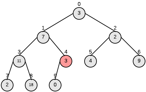
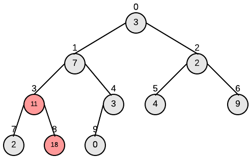


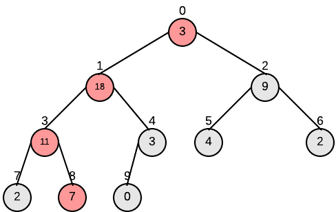
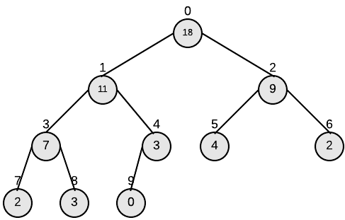
Heapsort(A)
到现在为止我们已经完成了2.2中构想的第一步,A[0]也就是root节点是数组中的最大值。如果直接将root节点取出,会破坏堆的结构,heapsort算法使用了一种非常聪明的方法。
+将root节点A[0]和堆中最后一个叶节点(leaf)进行交换,然后取出叶节点。这样,堆中除了以A[0]为root的树破坏了#2 - Heap Property,其他subtree仍然是最大堆。只需对A[0]进行Max-Heapify的操作。
+这个过程中将root节点取出的方法也很简单,只需将 heapsize←heapsize−1 。
下面是reference[1]中的Psudocode:
HEAPSORT(A):
    BUILD-MAX-HEAP(A)
     for i = A.length downto 1
       exchange A[0] with A[i]
       heapsize =  heapsize -1
       MAX-HEAPIFY(A , 0)
到此为止就是整个heapsort算法的流程了。注意,如果你是要闭眼睛也能写出一个堆排,最好的方法就是理解以上六个重要的操作。
Section 3 - runtime复杂度分析
这一个section,我们对heapsort算法过程中的操作进行复杂度分析。
首先一个总结:
- Max-Heapify ~ O(lgn)
- Build-Max-Heap ~ O(n)
- Heapsort ~ O(nlgn)
然后我们分析一下为什么是这样的。在以下的分析中,我们所指的所有节点 i 都是从1开始的。
Max-Heapify
这个不难推导,堆中任意节点 i 到叶节点的高度(height)是 lgn 。要专业的推导,可以参考使用master theorem。
Build-Max-Heap
在分析heapsort复杂度的时候,最有趣的就是这一步了。
如果堆的大小为 n ,那么堆的高度为 ⌊lgn⌋ ;
对于任意节点 i , i 到叶节点的高度是 h ,那么高度为 h 的的节点最多有 ⌈n/2h+1⌉ 个,下面是一个大概的直观证明:
-首先,一个大小为 n 的堆的叶节点(leaf)个数为 ⌈n/2⌉ :
--还记不记得最后一个有子节点的节点parent(length - 1)是第 ⌊n/2⌋ (注意这里不是java序号,是第几个),由此可证叶节点的个数为n - ⌊n/2⌋ ;
-那么如果去掉叶节点,剩下的堆的节点个数为 n−⌈n/2⌉=⌊n/2⌋ ,这个新树去掉叶节点后节点个数为 ⌊⌊n/2⌋/2⌋ ;
-(这需要好好想一想)以此类推,最后一个树的叶节点个数即为高度为 h 的节点的个数,一定小于 ⌈(n/2)/2h⌉ ,也就是 ⌈n/2h+1⌉ 。
对于任意节点 i , i 到叶节点的高度是 h ,运行Max-Heapify所需要的时间为 O(h) ,上面证明过。
那么Build-Max-Heap的上限时间为(参考reference[1]):
∑⌊lgn⌋h=0⌈n2h+1⌉O(h)=O(n∑⌊lgn⌋h=0h2h)
根据以下定理:
∑∞k=0kxk=x(1−x)2for|x|<1
我们用 x=12 替换求和的部分得到:
∑∞h=0h2h=1/2(1−1/2)2=2
综上所述,我们可以求得:
O(n∑⌊lgn⌋h=0h2h)=O(n∑∞h=0h2h)=O(2n)=O(n)
Heapsort
由于Build-Max-Heap复杂度为 O(n) ,有n-1次调用Max-Heapify(复杂度为 O(lgn) ),所有总的复杂度为 O(nlgn)
到此为止,所有functions的运行复杂度都分析完了,下面的章节就是使用Java的实现了。
Section 4 - Java Implementation
这个Section一共有两个内容,一个简单的Java实现(只有对key排序功能)和一个Priority Queue。
Parameters & Constructors:
protected double A[];
protected int heapsize;

//constructors
public MaxHeap(){}
public MaxHeap(double A[]){
    buildMaxHeap(A);
}
求parent/left child/right child:
protected int parent(int i) {return (i - 1) / 2;}
protected int left(int i) {return 2 * i + 1;}
protected int right(int i) {return 2 * i + 2;}
保持最大堆特性:
protected void maxHeapify(int i){
    int l = left(i);
    int r = right(i);
    int largest = i;
    if (l <= heapsize - 1 && A[l] > A[i])
        largest = l;
    if (r <= heapsize - 1 && A[r] > A[largest])
        largest = r;
    if (largest != i) {
        double temp = A[i];
        // swap
        A[i] = A[largest];
        A[largest] = temp;
        this.maxHeapify(largest);
    }
}
构造一个“最大堆”:
public void buildMaxHeap(double [] A){
    this.A = A;
    this.heapsize = A.length;

    for (int i = parent(heapsize - 1); i >= 0; i--)
        maxHeapify(i);
}
对一个array使用heapsort:
public void heapsort(double [] A){
    buildMaxHeap(A);

    int step = 1;
    for (int i = A.length - 1; i > 0; i--) {
        double temp = A[i];
        A[i] = A[0];
        A[0] = temp;
        heapsize--;
        System.out.println("Step: " + (step++) + Arrays.toString(A));
        maxHeapify(0);
    }
}
main函数:
public static void main(String[] args) {
    //a sample input
    double [] A = {3, 7, 2, 11, 3, 4, 9, 2, 18, 0};
    System.out.println("Input: " + Arrays.toString(A));
    MaxHeap maxhp = new MaxHeap();
    maxhp.heapsort(A);
    System.out.println("Output: " + Arrays.toString(A));

}
运行结果:
Input: [3.0, 7.0, 2.0, 11.0, 3.0, 4.0, 9.0, 2.0, 18.0, 0.0]
Step: 1[0.0, 11.0, 9.0, 7.0, 3.0, 4.0, 2.0, 2.0, 3.0, 18.0]
Step: 2[0.0, 7.0, 9.0, 3.0, 3.0, 4.0, 2.0, 2.0, 11.0, 18.0]
Step: 3[2.0, 7.0, 4.0, 3.0, 3.0, 0.0, 2.0, 9.0, 11.0, 18.0]
Step: 4[2.0, 3.0, 4.0, 2.0, 3.0, 0.0, 7.0, 9.0, 11.0, 18.0]
Step: 5[0.0, 3.0, 2.0, 2.0, 3.0, 4.0, 7.0, 9.0, 11.0, 18.0]
Step: 6[0.0, 3.0, 2.0, 2.0, 3.0, 4.0, 7.0, 9.0, 11.0, 18.0]
Step: 7[0.0, 2.0, 2.0, 3.0, 3.0, 4.0, 7.0, 9.0, 11.0, 18.0]
Step: 8[2.0, 0.0, 2.0, 3.0, 3.0, 4.0, 7.0, 9.0, 11.0, 18.0]
Step: 9[0.0, 2.0, 2.0, 3.0, 3.0, 4.0, 7.0, 9.0, 11.0, 18.0]
Step: 10[0.0, 2.0, 2.0, 3.0, 3.0, 4.0, 7.0, 9.0, 11.0, 18.0]
Output: [0.0, 2.0, 2.0, 3.0, 3.0, 4.0, 7.0, 9.0, 11.0, 18.0]
heapsort在实践中经常被一个实现的很好的快排打败,但heap有另外一个重要的应用,就是Priority Queue。这篇文章只做拓展内容提及,简单得说,一个priority queue就是一组带key的element,通过key来构造堆结构。通常,priority queue使用的是min-heap,例如按时间顺序处理某些应用中的objects。
为了方便,我用Inheritance实现一个priority queue:
package heapsort;

import java.util.Arrays;

public class PriorityQueue extends MaxHeap{

    public PriorityQueue(){super();}
    public PriorityQueue(double [] A){super(A);}

    public double maximum(){
        return A[0];
    }

    public double extractMax(){
        if(heapsize<1)
            System.err.println("no element in the heap");
        double max = A[0];
        A[0] = A[heapsize-1];
        heapsize--;
        this.maxHeapify(0);
        return max;
    }

    public void increaseKey(int i,double key){
        if(key < A[i])
            System.err.println("new key should be greater than old one");

        A[i] = key;
        while(i>0 && A[parent(i)] <A[i]){
            double temp = A[i];
            A[i] = A[parent(i)];
            A[parent(i)] = temp;
            i = parent(i);
        }
    }

    public void insert(double key){
        heapsize++;
        A[heapsize - 1] = Double.MIN_VALUE;
        increaseKey(heapsize - 1, key);
    }

    public static void main(String[] args) {
        //a sample input
        double [] A = {3, 7, 2, 11, 3, 4, 9, 2, 18, 0};
        System.out.println("Input: " + Arrays.toString(A));
        PriorityQueue pq = new PriorityQueue();
        pq.buildMaxHeap(A);
        System.out.println("Output: " + Arrays.toString(A));
        pq.increaseKey(2, 100);
        System.out.println("Output: " + Arrays.toString(A));
        System.out.println("maximum extracted: " + pq.extractMax());
        pq.insert(33);
        System.out.println("Output: " + Arrays.toString(A));

    }
}

priorityqueue
运行结果:
Input: [3.0, 7.0, 2.0, 11.0, 3.0, 4.0, 9.0, 2.0, 18.0, 0.0]
Output: [18.0, 11.0, 9.0, 7.0, 3.0, 4.0, 2.0, 2.0, 3.0, 0.0]
Output: [100.0, 11.0, 18.0, 7.0, 3.0, 4.0, 2.0, 2.0, 3.0, 0.0]
maximum extracted: 100.0
Output: [33.0, 18.0, 4.0, 7.0, 11.0, 0.0, 2.0, 2.0, 3.0, 3.0]
Section 5 - 小结
首先要说本文全部是原创,如需要使用,只需要引用一下并不需要通知我。
写到最后发现有很多写得很冗余,也有啰嗦的地方。感觉表达出来对自己的知识巩固很有帮助。Heapsort真是一个非常有意思的排序方法,是一个通用而不算复杂的算法,这是决定开始写blogs后的第一篇文章,一定有很多不足,欢迎讨论!之后打算写一些机器学习和计算机视觉方面的来抛砖引玉。希望通过博客园这个平台可以交到更多有钻研精神的朋友。
Bibliography
[1] Thomas H. Cormen, Charles E. Leiserson, Ronald L. Rivest, and Clifford Stein.
Introduction to Algorithms. MIT Press, 3rd edition, 2009.
[2] Wikipedia. Heapsort — wikipedia, the free encyclopedia, 2014. [Online; accessed
15-September-2014].