测试一张自定义的手写体数字
上面已经进行了mnist数据的训练,也对测试数据进行的测试,准确率在99%左右。那么如果我们想自己测一下一张字节手写的数字,看看他学习的是否准确,改怎么利用caffemodel权值文件呢。
下面就来测试一张自定义的手写体数字。
利用模型lenet_iter_10000.caffemodel测试单张手写体数字所需要的文件:
(1)待测试图片(自己画的也行,网络上下的也行);需要注意的是,不管是什么格式,都要转换为28*28大小的黑白灰度图像,具体转化方法请自行百度,不想转化也可以从这个链接下载,下载链接: https://pan.baidu.com/s/1Ck6l7bAncK2BpcqWXG67Dg 密码:csig,这些图片是网上已经转好的。
(2)deploy.prototxt(模型描述型文件);
(3)network.caffemodel(模型权值文件),在本例中就是lenet_iter_10000.caffemodel
(4)labels.txt(标签文件),本利中是synset_words.txt文件;
(5)mean.binaryproto(二进制图像均值文件);
(6)classification.bin(二进制程序名)。与二进制均值文件配合使用,只是均值文件不同的模型有不同的均值文件,而这个bin文件为通用的,就是任何模型都可以做分类使用。
1.准备一张自定义的图片
下载链接中的图片,拷贝到caffe/examples/mnist/目录下。
2.生成deploy.prototxt文件
deploy.prototxt文件的作用和lenet_train_test.prototxt文件类似,或者说对后者改动可得到前者。在熟悉生成文件的原理及方法之后我们可以之间在原训练prototxt网络文件中改动。在examples/mnist目录下复制一份lenet_train_test.prototxt修改并保存后得到deploy.prototxt如下:
name: "LeNet"


layer {
  name:"data"
 type: "Input"
 top: "data"
 input_param { shape: { dim: 1 dim: 1 dim: 28 dim: 28 } }
}


layer {
  name:"conv1"
 type: "Convolution"
 bottom: "data"
 top: "conv1"
 convolution_param {
   num_output: 20
   kernel_size: 5
   stride: 1
   weight_filler {
     type: "xavier"
   }
 }
}
layer {
  name:"pool1"
 type: "Pooling"
 bottom: "conv1"
 top: "pool1"
 pooling_param {
   pool: MAX
   kernel_size: 2
   stride: 2
  }
}
layer {
  name:"conv2"
 type: "Convolution"
 bottom: "pool1"
 top: "conv2"
 convolution_param {
   num_output: 50
   kernel_size: 5
   stride: 1
   weight_filler {
     type: "xavier"
   }
 }
}
layer {
  name:"pool2"
 type: "Pooling"
 bottom: "conv2"
 top: "pool2"
 pooling_param {
   pool: MAX
   kernel_size: 2
   stride: 2
  }
}
layer {
  name:"ip1"
 type: "InnerProduct"
 bottom: "pool2"
 top: "ip1"
 inner_product_param {
   num_output: 500
   weight_filler {
     type: "xavier"
   }
 }
}
layer {
  name:"relu1"
 type: "ReLU"
 bottom: "ip1"
 top: "ip1"
}
layer {
  name:"ip2"
 type: "InnerProduct"
 bottom: "ip1"
 top: "ip2"
 inner_product_param {
   num_output: 10
   weight_filler {
     type: "xavier"
   }
 }
}


layer {
  name:"prob"
 type: "Softmax"
 bottom: "ip2"
 top: "prob"
}
当然,也可以采用代码的方式来自动生成该deploy.prototxt文件 。deploy文件没有第一层数据输入层,也没有最后的Accuracy层,但最后多了一个Softmax概率层。
deploy.py代码如下;
# -*- coding: utf-8 -*-

from caffe  import layers as L,params as P,to_proto
root='/root/caffe/'
deploy=root+'examples/mnist/deploy.prototxt'    #文件保存路径

def create_deploy():
    #少了第一层,data层
    conv1=L.Convolution(name='conv1',bottom='data', kernel_size=5, stride=1,num_output=20, pad=0,weight_filler=dict(type='xavier'))
    pool1=L.Pooling(conv1,name='pool1',pool=P.Pooling.MAX, kernel_size=2, stride=2)
    conv2=L.Convolution(pool1, name='conv2',kernel_size=5, stride=1,num_output=50, pad=0,weight_filler=dict(type='xavier'))
    pool2=L.Pooling(conv2, name='pool2', pool=P.Pooling.MAX, kernel_size=2, stride=2)
    fc3=L.InnerProduct(pool2, name='ip1',num_output=500,weight_filler=dict(type='xavier'))
    relu3=L.ReLU(fc3, name='relu1',in_place=True)
    fc4 = L.InnerProduct(relu3, name='ip2',num_output=10,weight_filler=dict(type='xavier'))
    #最后没有accuracy层,但有一个Softmax层
    prob=L.Softmax(fc4, name='prob')
    return to_proto(prob)
def write_deploy():
    with open('deploy.prototxt', 'w+') as f:
        f.write('name:"LeNet"\n')
        f.write('layer {\n')
        f.write('name:"data"\n')
        f.write('type:"Input"\n')
        f.write('top:"data"\n')
        f.write('input_param { shape : {')
        f.write('dim:1 ')
        f.write('dim:1 ')
        f.write('dim:28 ')
        f.write('dim:28 ')
        f.write('} } }\n\n')
        f.write(str(create_deploy()))
if __name__ == '__main__':
    write_deploy()
3.network.caffemodel(模型权值文件)
network.caffemodel在训练时已经生成,在本例中就是lenet_iter_10000.caffemodel文件。
4.生成labels.txt标签文件
在当前目录下新建一个txt文件,命名为synset_words.txt,里面内容为我们训练mnist的图片内容,共有0~9十个数,那么我们就建立如下内容的标签文件:

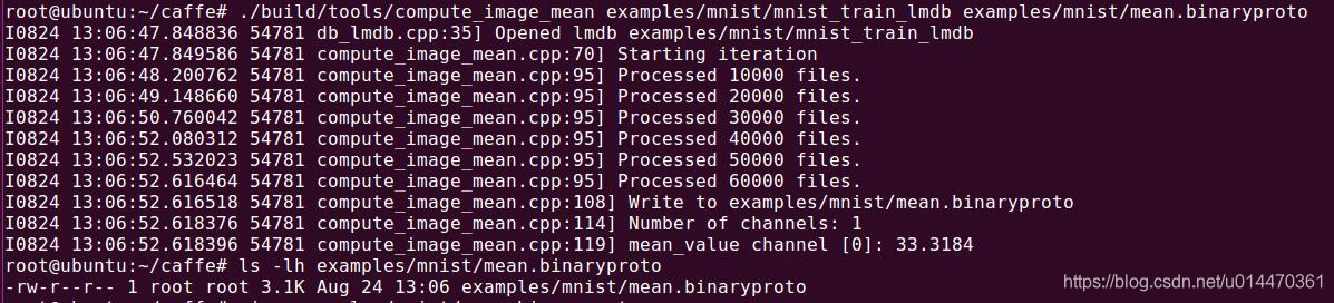
5.生成mean.binaryproto二进制均值文件
均值文件分为二进制均值文件和python类均值文件。
caffe作者为我们提供了一个计算均值的文件compute_image_mean.cpp,放在caffe根目录下的tools文件夹里面,运行下面命令生成mean.binaryproto二进制均值文件。
build/tools/compute_image_mean  \
examples/mnist/mnist_train_lmdb \
examples/mnist/mean.binaryproto
6.利用classification.bin二进制程序进行测试
在example文件夹中有一个cpp_classification的文件夹,打开它,有一个名为classification的cpp文件,这就是caffe提供给我们的调用分类网络进行前向计算,得到分类结果的接口。就是这个文件在命令中会得到classification.bin。
使用下面的指令开始测试自定义的一个数字图片:
./build/examples/cpp_classification/classification.bin \
examples/mnist/deploy.prototxt \
examples/mnist/lenet_iter_10000.caffemodel \
examples/mnist/mean.binaryproto \
examples/mnist/synset_words.txt \
examples/mnist/picture/0.0.jpg
测试结果:
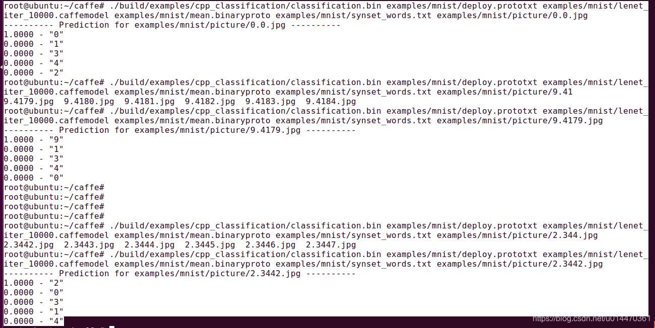
可以看到,测试0时输出的0标签对应的是1.0000,测试9时输出的9标签对应的是1.0000,测试2时输出的2标签对应的是1.0000,结果还是很准的。
绘制loss图
在上一篇mnist训练的过程中,不停的打印了一些训练的速度,学习率,loss值等。那么有没有图片的形式可以更直观的反应训练过程中loss和准确率的变化趋势呢?
当然是有的,需要编写一个pyton程序loss.py。参考网上的一个例程:
# -*- coding: utf-8 -*-
import numpy as np #导入numpy库并命名为np,numpy支持大量的维度数组与矩阵运算,此外也针对数组运算提供大量的数学函数库。
import matplotlib.pyplot as plt #导入matplotlib.pyplot库并命名为plt,Matplotlib 是 Python 的绘图库。 matplotlib可与 NumPy 一起使用,提供了一种有效的 MatLab 开源替代方案
import sys,os  #导入sys模块,sys模块包含了与Python解释器和它的环境有关的函数;导入os模块,os模块里面有环境变量的映射关系,目录等
caffe_root = '/root/caffe'
sys.path.insert(0,caffe_root+'python')  #sys.path为一个列表,用insert直接插到首位,插入python的环境变量
import caffe

caffe.set_mode_cpu() #设置caffe  cpu运行模式
solver = caffe.SGDSolver('/root/caffe/examples/mnist/lenet_solver.prototxt')
# 执行完上面的语句以后,网络的相应的权值与偏置会根据我们的定义进行赋值的

niter=1000  #迭代1000次
test_interval = 200  #200次测试一次
train_loss = np.zeros(niter) #1维,大小为1000的数组
#np.zeros返回一个给定形状和类型的用0填充的数组,本例为array([ 0,  0,  0,  0,  0 ......]),长度是1000
test_acc = np.zeros(int(np.ceil(niter / test_interval)))#1维,大小为5的数组
#np.ceil() 计算大于等于该值的最小整数,本例niter / test_interval,np.ceil(5)是5

for it in range(niter):
	solver.step(1)
	# solver.net.forward() , solver.test_nets[0].forward() 和 solver.step(1) 区别和作用。
	#三个函数都是将批量大小(batch_size)的图片送到网络,
	#solver.net.forward() 和 solver.test_nets[0].forward() 是将batch_size个图片送到网络中去,只有前向传播(Forward Propagation,BP),solver.net.forward()作用于训练集,solver.test_nets[0].forward() 作用于测试集,一般用于获得测试集的正确率。
	#solver.step(1) 也是将batch_size个图片送到网络中去,不过 solver.step(1) 不仅有FP,而且还有反向传播(Back Propagation,BP)!这样就可以更新整个网络的权值(weights),同时得到该batch的loss。


	train_loss[it] = solver.net.blobs['loss'].data # 获取每一次迭代的loss值
	solver.test_nets[0].forward(start='conv1')   #表示从conv1开始,这样的话,data层不用传新的数据了。

	if it % test_interval == 0:
		acc=solver.test_nets[0].blobs['accuracy'].data  #获取test_interval整数倍时的准确率
		#solver.net.blobs为一个字典的数据类型,里面的key值为各个layer 的名字,value为caffe的blob块
		print 'Iteration',it,'testing...','accuracy:',acc
		test_acc[it // test_interval] = acc  #      //是整除运算符,取整数部分

print test_acc
_,ax1= plt.subplots()
ax2= ax1.twinx()#matplotlib:次坐标轴ax2=ax1.twinx(),产生一个ax1的镜面坐标
ax1.plot(np.arange(niter),train_loss)
ax2.plot(test_interval * np.arange(len(test_acc)),test_acc,'r')
ax1.set_xlabel('iteration')
ax1.set_ylabel('train loss')
ax2.set_ylabel('test accuracy')
plt.savefig("mnist_loss.png")
plt.show()
loss.py程序的详细解析见上面。
运行绘制
python loss.py
执行loss.py后,就开始训练了,这里我训练了1000次,200次输出一次测试。
loss曲线图如下:
eog mnist_loss.png
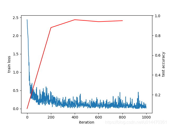
如上图,可以看到loss随着训练次数的增加,呈现出逐渐震荡收敛的,loss 值呈现下降趋势,准确率在不断的上升。
备注:
_,ax1= plt.subplots() 这一句中为什么开头有 _,这俩字符,查了一圈资料也没明白,有知道的还请告知一下~