建模与调参_代码示例部分
# 导入工具包
import pandas as pd
import numpy as np
import warnings
warnings.filterwarnings('ignore')   # 代码可以正常运行但是会提示警告,很烦人,有了这行代码就能忽略警告了
pd.set_option('display.max_columns', None)      # 显示所有列
# 创建一个reduce_mem_usage函数,通过调整数据类型,减少数据在内存中占用的空间
def reduce_mem_usage(df):
    '''
    遍历DataFrame的所有列并修改它们的数据类型以减少内存使用
    :param df: 需要处理的数据集
    :return:
    '''
    start_mem = df.memory_usage().sum()     # 记录原数据的内存大小
    print('Memory usage of dataframe is{:.2f} MB'.format(start_mem))

    for col in df.columns:
        col_type = df[col].dtypes

        if col_type != object:      # 这里只过滤了object格式,如果代码中还包含其他类型,要一并过滤
            c_min = df[col].min()
            c_max = df[col].max()
            if str(col_type)[:3] == 'int':      # 如果是int类型的话,不管是int64还是int32,都加入判断
                # 依次尝试转化成in8,in16,in32,in64类型,如果数据大小没溢出,那么转化
                if c_min > np.iinfo(np.int8).min and c_max < np.iinfo(np.int8).max:
                    df[col] = df[col].astype(np.int8)
                elif c_min > np.iinfo(np.int16).min and c_max < np.iinfo(np.int16).max:
                    df[col] = df[col].astype(np.int16)
                elif c_min > np.iinfo(np.int32).min and c_max < np.iinfo(np.int32).max:
                    df[col] = df[col].astype(np.int32)
                elif c_min > np.iinfo(np.int64).min and c_max < np.iinfo(np.int64).max:
                    df[col] = df[col].astype(np.int64)
            else:                               # 不是整形的话,那就是浮点型
                if c_min > np.finfo(np.float16).min and c_max < np.finfo(np.float16).max:
                    df[col] = df[col].astype(np.float16)
                elif c_min > np.finfo(np.float32).min and c_max < np.finfo(np.float32).max:
                    df[col] = df[col].astype(np.float32)
                else:
                    df[col] = df[col].astype(np.float64)
        else:   # 如果不是数值型的话,转化成category类型
            df[col] = df[col].astype('category')

    end_mem = df.memory_usage().sum()   # 看一下转化后的数据的内存大小
    print('Memory usage after optimization is {:.2f} MB'.format(end_mem))
    print('Decreased by {:.1f}%'.format(100 * (start_mem - end_mem) / start_mem))   # 看一下压缩比例
    return df
# 读取我们为树模型准备的特征数据,并且将数据压缩
sample_feature = reduce_mem_usage(pd.read_csv(r'F:\Users\TreeFei\文档\PyC\ML_Used_car\data\data_for_tree.csv'))

Memory usage of dataframe is60507376.00 MB
Memory usage after optimization is 15724155.00 MB
Decreased by 74.0%
数据内存大小压缩了74%,看来效果拔群
# 把我们需要用的特征挑出(仅仅是列名,用来分离特征集和标签集)
continuous_feature_names = [x for x in sample_feature.columns if x not in ['price', 'brand', 'model']]
# 处理一下sample_feature数据集的缺失值
sample_feature = sample_feature.dropna().replace('-', 0).reset_index(drop=True)
这里我比较疑惑为什么replace了’-’?
然后我看了看数据
sample_feature[sample_feature.isin(['-'])]
发现每非常多的样本都存在’-’,说明有一个特征里面有’-’
我第一时间考虑到了notRepairedDamage这个特征,因为它是唯一一个object类型的特征
sample_feature['notRepairedDamage']
果不其然,它是个类别特征,Categories (3, object): [-, 0.0, 1.0],有三个类别:’-’, ‘0’, ‘1’
# 既然想起来了notRepairedDamage不是数值型特征,那么我们把它转化一下
sample_feature['notRepairedDamage'] = sample_feature['notRepairedDamage'].astype(np.float32)
# 处理完了之后,我们拿出我们挑选的特征和它的价格构造训练集
train = sample_feature[continuous_feature_names + ['price']]

train_X = train[continuous_feature_names]
train_y = train['price']
# 简单建模
from sklearn.linear_model import LinearRegression       # 线性回归模型 y = wx + b
'''
这里比较疑惑,不是说用树模型嘛?挑的也是树模型的数据,为啥这里建了LR,看看再说
'''
model = LinearRegression(normalize=True)    # normalize参数决定是否将数据归一化
model = model.fit(train_X, train_y)
# 查看训练的lR模型的截距(intercept)与权重(coef)
'intercept:' + str(model.intercept_)
'''
zip() - 可以将两个可迭代的对象,组合返回成一个元组数据
dict() - 使用元组数据构建字典
items方法 - items() 函数以列表返回可遍历的(键, 值) 元组数组
sort(iterable, cmp, key, reverse) - 排序函数
    iterable - 指定要排序的list或者iterable
    key - 指定取待排序元素的哪一项进行排序 - 这里x[1]表示按照列表中第二个元素排序
    reverse - 是一个bool变量,表示升序还是降序排列,默认为False(升序)
'''
sorted(dict(zip(continuous_feature_names, model.coef_)).items(), key=lambda x: x[1], reverse=True)
# 这行代码返回了每个特征的权重,按照权重降序排列

import matplotlib.pyplot as plt
'''
np.random.randint() - 产生离散均匀分布的整数
            取数范围:若high不为None时,取[low,high)之间随机整数,否则取值[0,low)之间随机整数
            size - 54输出的大小,可以是整数也可以是元组
'''
subsample_index = np.random.randint(low=0, high=len(train_y), size=50)  # 随机生成0-50000之间的50个整数
# 绘制v_9的值与标签的散点图
plt.scatter(train_X['v_9'][subsample_index], train_y[subsample_index], color='black')
plt.scatter(train_X['v_9'][subsample_index], model.predict(train_X.loc[subsample_index]), color='blue')
plt.xlabel('v_9')
plt.ylabel('price')
plt.legend(['True Price', 'Predicted'], loc='upper right')
print('The predicted price is obvious different from true price')
plt.show()

我们发现预测点和真实值差别较大,且有预测值出现了结果为负的情况,不符合实际情况,模型有问题
# 我们看一下价格的分布图
import seaborn as sns
print('It is clear to see the price shows a typical exponential distribution')
plt.figure(figsize=(15, 5))
plt.subplot(1, 2, 1)
sns.distplot(train_y)

价格呈长尾分布,不利于建模预测,因为很多模型都假设数据误差项符合正态分布
plt.subplot(1, 2, 2)
'''
np.quantile(train_y, 0.9) - 求train_y 的90%的分位数
下面这个代码是把价格大于90%分位数的部分截断了,就是长尾分布截断
'''
sns.distplot(train_y[train_y < np.quantile(train_y, 0.9)])

看上去好多了
# 为了更加贴近正态分布,对price进行log(x+1)变换
train_y_In = np.log(train_y + 1)

print('The transformed price seems like normal distribution')
plt.figure(figsize=(15, 5))
plt.subplot(1, 2, 1)
sns.distplot(train_y_In)
plt.subplot(1, 2, 2)
sns.distplot(train_y_In[train_y_In < np.quantile(train_y_In, 0.9)])

这回看上去像正态分布了,右边的图是做了长尾截断处理
# 我们再训练一次
model = model.fit(train_X, train_y_In)
print('intercept:' + str(model.intercept_))
sorted(dict(zip(continuous_feature_names, model.coef_)).items(), key=lambda x: x[1], reverse=True)
# 可视化一波,还是看v_9
plt.scatter(train_X['v_9'][subsample_index], train_y[subsample_index], color='black')
'''
np.exp() - 求e的幂次方,因为训练模型的时候log变换了,所以预测完了对比结果的时候得变回来
'''
plt.scatter(train_X['v_9'][subsample_index], np.exp(model.predict(train_X.loc[subsample_index])), color='blue')
plt.xlabel('v_9')
plt.ylabel('price')
plt.legend(['True Price', 'Predicted'], loc='upper right')
plt.show()

看上去准多了,预测值和真实值更加贴合
# 五折交叉验证
from sklearn.model_selection import cross_val_score
from sklearn.metrics import mean_absolute_error, make_scorer
定义一个函数,用来处理预测值和真实值的log变换
'''
numpy.nan_to_num(x) - 使用0代替数组x中的nan元素,使用有限的数字代替inf元素
'''


def log_transfer(func):
    def warpper(y, yhat):
        result = func(np.log(y), np.nan_to_num(np.log(yhat)))
        return result
    return warpper
# 我们使用线性回归模型,对未处理过标签的特征数据做5折交叉验证
scores = cross_val_score(model, X=train_X, y=train_y, verbose=1, cv=5,
                         scoring=make_scorer(log_transfer(mean_absolute_error)))
'''
verbose - 日志显示
            verbose = 0 为不在标准输出流输出日志信息
            verbose = 1 为输出进度条记录
            verbose = 2 为每个epoch输出一行记录

make_scorer() - 工厂函数,自己定评分标准
这里的log_transfer()是返回log化的标签预测值和真实值
'''
print('AVG:', np.mean(scores))
— AVG: 1.3654295934396061 —> 5次的MAE平均值
# 我们再使用线性回归模型,对处理过标签的特征数据做5折交叉验证
scores_In = cross_val_score(model, X=train_X, y=train_y_In, verbose=1, cv=5,
                         scoring=make_scorer(mean_absolute_error))
print('AVG:', np.mean(scores_In))
— AVG: 0.1932330179438017
MAE从1.365降低到0.193,误差缩小了很多
# 事实上,五折交叉验证在某些与时间相关的数据集上反而反映了不真实的情况
用2018年的二手车价格预测2017年是不合理的,所以我们可以用时间靠前的4/5样本当作训练集,靠后的1/5当验证集
import datetime     # 这里我没看到datetime的作用,只能认为数据集是按照时间排列的
sample_feature = sample_feature.reset_index(drop=True)      # 重置索引
split_point = len(sample_feature) // 5 * 4      # 设置分割点

train = sample_feature.loc[:split_point].dropna()
val = sample_feature.loc[split_point:].dropna()

train_X = train[continuous_feature_names]
train_y_In = np.log(train['price'] + 1)
val_X = val[continuous_feature_names]
val_y_In = np.log(val['price'] + 1)

model = model.fit(train_X, train_y_In)
mean_absolute_error(val_y_In, model.predict(val_X))
— MAE为0.196,和五折交叉验证差别不大
# 绘制学习率曲线与验证曲线
from sklearn.model_selection import learning_curve, validation_curve
创建绘制学习率曲线的函数
def plot_learning_curve(estimator, title, X, y, ylim=None, cv=None, n_jobs=1, train_sizes=np.linspace(.1, 1.0, 5)):
    plt.figure()
    plt.title(title)
    if ylim is not None:
        plt.ylim(*ylim)     # 如果规定了ylim的值,那么ylim就用规定的值
    plt.xlabel('Training example')
    plt.ylabel('score')
    train_size, train_scores, test_scores = learning_curve(estimator, X, y, cv=cv, n_jobs=n_jobs,
                                                           train_sizes=train_sizes,
                                                           scoring=make_scorer(mean_absolute_error))
    train_scores_mean = np.mean(train_scores, axis=1)
    train_scores_std = np.std(train_scores, axis=1)
    test_scores_mean = np.mean(test_scores, axis=1)
    test_scores_std = np.std(test_scores, axis=1)
    plt.grid()
    '''
    fill_between()
            train_sizes - 第一个参数表示覆盖的区域
            train_scores_mean - train_scores_std - 第二个参数表示覆盖的下限
            train_scores_mean + train_scores_std - 第三个参数表示覆盖的上限
            color - 表示覆盖区域的颜色
            alpha - 覆盖区域的透明度,越大越不透明 [0,1]
    '''
    plt.fill_between(train_sizes, train_scores_mean - train_scores_std,
                     train_scores_mean + train_scores_std, alpha=0.1, color='r')
    plt.fill_between(train_sizes, test_scores_mean - test_scores_std,
                     test_scores_mean + test_scores_std)
    plt.plot(train_sizes, train_scores_mean, 'o-', color='r', label='Training score')
    plt.plot(train_sizes, test_scores_mean, 'o-', color='g', label='Cross-validation score')
    plt.legend(loc='best')
    return plt

plot_learning_curve(LinearRegression(), 'Liner_model', train_X[:1000], train_y_In[:1000],
                    ylim=(0.0, 0.5), cv=5, n_jobs=1)

模型在训练集拟合的不错,在验证集中表现一般
# 嵌入式特征选择 - 大部分情况下都是用嵌入式做特征选择
1.L1正则化 - Lasso回归 -
模型被限制在正方形区域(二维区域下),损失函数的最小值往往在正方形(约束)的角上,很多权值为0(多维),所以可以实现模型的稀疏性(生成稀疏权值矩阵,进而用于特征选择
2.L2正则化 - 岭回归 -
模型被限制在圆形区域(二维区域下),损失函数的最小值因为圆形约束没有角,所以不会使得权重为0,但是可以使得权重都尽可能的小,最后得到一个所有参数都比较小的模型,这样模型比较简单,能适应不同数据集,一定程度上避免了过拟合
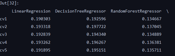
# 我们看下三种模型的效果对比:线性回归; 加入了L1的Lasso回归; 加入了L2的岭回归
from sklearn.linear_model import Ridge
from sklearn.linear_model import Lasso
models = [LinearRegression(), Ridge(), Lasso()]
result = dict()     # 创建一个用来装结果的字典
for model in models:
    model_name = str(model).split('(')[0]   # 把括号去掉,只保留名字
    scores = cross_val_score(model, X=train_X, y=train_y_In, verbose=0, cv=5,       # 五折交叉验证
                             scoring=make_scorer(mean_absolute_error))
    result[model_name] = scores
    print(model_name + ' is finished')

result = pd.DataFrame(result)
result.index = ['cv' + str(x) for x in range(1, 6)]
result

model_Lr = LinearRegression().fit(train_X, train_y_In)
print('intercept:' + str(model_Lr.intercept_))
sns.barplot(abs(model_Lr.coef_), continuous_feature_names)

— 线性回归模型:发现v_6, v_8, v_9权重大
model_Ridge = Ridge().fit(train_X, train_y_In)
print('intercept:' + str(model_Ridge.intercept_))
sns.barplot(abs(model_Ridge.coef_), continuous_feature_names)

— 岭回归:发现有更多的参数对模型起到影响,而且参数都比较小,一定程度上避免了过拟合现象,抗扰动能力强
model_Lasso = Lasso().fit(train_X, train_y_In)
print('intercept:' + str(model_Lasso.intercept_))
sns.barplot(abs(model_Lasso.coef_), continuous_feature_names)

— lasso回归:发现power和used_time这两个特征很重要,L1正则化有助于生成一个稀疏权值矩阵,进而用于特征选择
# 看看常用的非线性模型,与线性模型的效果进行一个比对
'''
SVM - 支持向量机 - 通过寻求结构化风险最小来提高学习机泛化能力,基本模型定义为特征空间上的间隔最大的线性分类器
                    支持向量机的学习策略便是间隔最大化
    SVR - 用于标签连续值的回归问题
    SVC - 用于分类标签的分类问题
'''
from sklearn.svm import SVC     # 这里用SVR是不是好得多?
from sklearn.tree import DecisionTreeRegressor      # 决策树回归
from sklearn.ensemble import RandomForestRegressor  # 随机森林回归

'''
Boosting算法思想 -  一堆弱分类器的组合就可以成为一个强分类器;
                    不断地在错误中学习,迭代来降低犯错概率
                    通过一系列的迭代来优化分类结果,每迭代一次引入一个弱分类器,来克服现在已经存在的弱分类器组合的短板

        Adaboost      - 整个训练集上维护一个分布权值向量W
                        用赋予权重的训练集通过弱分类算法产生分类假设(基学习器)y(x)
                        然后计算错误率,用得到的错误率去更新分布权值向量w
                        对错误分类的样本分配更大的权值,正确分类的样本赋予更小的权值
                        每次更新后用相同的弱分类算法产生新的分类假设,这些分类假设的序列构成多分类器
                        对这些多分类器用加权的方法进行联合,最后得到决策结果

        Gradient Boosting - 迭代的时候选择梯度下降的方向来保证最后的结果最好
                            损失函数用来描述模型的'靠谱'程度,假设模型没有过拟合,损失函数越大,模型的错误率越高
                            如果我们的模型能够让损失函数持续的下降,最好的方式就是让损失函数在其梯度方向下降

                            GradientBoostingRegressor()
                                    loss - 选择损失函数,默认值为ls(least squres),即最小二乘法,对函数拟合
                                    learning_rate - 学习率
                                    n_estimators - 弱学习器的数目,默认值100
                                    max_depth - 每一个学习器的最大深度,限制回归树的节点数目,默认为3
                                    min_samples_split - 可以划分为内部节点的最小样本数,默认为2
                                    min_samples_leaf - 叶节点所需的最小样本数,默认为1
参考资料:https://www.cnblogs.com/zhubinwang/p/5170087.html
'''
from sklearn.ensemble import GradientBoostingRegressor

'''
MLPRegressor  - 人工神经网络,了解的不多
参数详解
    hidden_layer_sizes - hidden_layer_sizes=(50, 50),表示有两层隐藏层,第一层隐藏层有50个神经元,第二层也有50个神经元
    activation - 激活函数   {‘identity’, ‘logistic’, ‘tanh’, ‘relu’},默认relu
                identity - f(x) = x
                logistic - 其实就是sigmod函数,f(x) = 1 / (1 + exp(-x))
                tanh - f(x) = tanh(x)
                relu - f(x) = max(0, x)
    solver - 用来优化权重     {‘lbfgs’, ‘sgd’, ‘adam’},默认adam,
                lbfgs - quasi-Newton方法的优化器:对小数据集来说,lbfgs收敛更快效果也更好
                sgd - 随机梯度下降
                adam - 机遇随机梯度的优化器
    alpha - 正则化项参数,可选的,默认0.0001
    learning_rate - 学习率,用于权重更新,只有当solver为’sgd’时使用
    max_iter - 最大迭代次数,默认200
    shuffle - 判断是否在每次迭代时对样本进行清洗,默认True,只有当solver=’sgd’或者‘adam’时使用
'''
from sklearn.neural_network import MLPRegressor

'''
XGBRegressor - 梯度提升回归树,也叫梯度提升机

                采用连续的方式构造树,每棵树都试图纠正前一棵树的错误
                与随机森林不同,梯度提升回归树没有使用随机化,而是用到了强预剪枝
                从而使得梯度提升树往往深度很小,这样模型占用的内存少,预测的速度也快
'''
from xgboost.sklearn import XGBRegressor
from lightgbm.sklearn import LGBMRegressor

models = [LinearRegression(), DecisionTreeRegressor(), RandomForestRegressor(),
          GradientBoostingRegressor(), MLPRegressor(solver='lbfgs', max_iter=100),
          XGBRegressor(n_estimators=100, objective='reg:squarederror'),
          LGBMRegressor(n_estimators=100)]

result = dict()
for model in models:
    model_name = str(model).split('(')[0]
    scores = cross_val_score(model, X=train_X, y=train_y_In,
                             verbose=0, cv=5, scoring=make_scorer(mean_absolute_error))
    result[model_name] = scores
    print(model_name + ' is finished')

result = pd.DataFrame(result)
result.index = ['cv' + str(x) for x in range(1, 6)]
result

整体看来,随机森林在每一折的表现最好,XGB也不错,LGB最小值在0.143左右
# 模型调参-以LGB - LGBMRegressor为例
''''
LightGBM - 使用的是histogram算法,占用的内存更低,数据分隔的复杂度更低
            思想是将连续的浮点特征离散成k个离散值,并构造宽度为k的Histogram
            然后遍历训练数据,统计每个离散值在直方图中的累计统计量
            在进行特征选择时,只需要根据直方图的离散值,遍历寻找最优的分割点

            LightGBM采用leaf-wise生长策略:
            每次从当前所有叶子中找到分裂增益最大(一般也是数据量最大)的一个叶子,然后分裂,如此循环。
            因此同Level-wise相比,在分裂次数相同的情况下,Leaf-wise可以降低更多的误差,得到更好的精度
            Leaf-wise的缺点是可能会长出比较深的决策树,产生过拟合
            因此LightGBM在Leaf-wise之上增加了一个最大深度的限制,在保证高效率的同时防止过拟合
'''

'''
参数:
num_leaves - 控制了叶节点的数目,它是控制树模型复杂度的主要参数,取值应 <= 2 ^(max_depth)
bagging_fraction - 每次迭代时用的数据比例,用于加快训练速度和减小过拟合
feature_fraction - 每次迭代时用的特征比例,例如为0.8时,意味着在每次迭代中随机选择80%的参数来建树,
                    boosting为random forest时用
min_data_in_leaf - 每个叶节点的最少样本数量。
                    它是处理leaf-wise树的过拟合的重要参数
                    将它设为较大的值,可以避免生成一个过深的树。但是也可能导致欠拟合
max_depth - 控制了树的最大深度,该参数可以显式的限制树的深度
n_estimators - 分多少颗决策树(总共迭代的次数)

objective - 问题类型
            regression - 回归任务,使用L2损失函数
            regression_l1 - 回归任务,使用L1损失函数
            huber - 回归任务,使用huber损失函数
            fair - 回归任务,使用fair损失函数
            mape (mean_absolute_precentage_error) - 回归任务,使用MAPE损失函数
'''
## 贪心算法
– LGB的参数集合
objective = ['regression', 'regression_l1', 'mape', 'huber', 'fair']

num_leaves = [3, 5, 10, 15, 20, 40, 55]
max_depth = [3, 5, 10, 15, 20, 40, 55]
bagging_fraction = []
feature_fraction = []
drop_rate = []
贪心调参
'''
建立数学模型来描述问题
把求解的问题分成若干个子问题
对每个子问题求解,得到子问题的局部最优解
把子问题的解局部最优解合成原来问题的一个解
总是做出在当前看来是最好的选择,也就是说,不从整体最优上加以考虑,它所做出的仅仅是在某种意义上的局部最优解

对于一个具体问题,要确定它是否具有贪心选择性质,必须证明每一步所作的贪心选择最终导致问题的整体最优解
'''
# 局部最优解 - objective
best_obj = dict()
for obj in objective:
    model = LGBMRegressor(objective=obj)
    score = np.mean(cross_val_score(model, X=train_X, y=train_y_In, verbose=0,
                                    cv=5, scoring=make_scorer(mean_absolute_error)))
    best_obj[obj] = score

# 局部最优解 - num_leaves    --- 此时得限制objective参数,得是mae值最小,即误差最小的那个问题类型
best_leaves = dict()
for leaves in num_leaves:
    '''
    best_obj.items() - 把best_obj字典中的元组装进列表
    key=lambda x: x[1] - 取前一个对象的第二维的数据,即原字典的value值
    min(best_obj.items(), key=lambda x: x[1]) - 选择best_obj中value值最小的那组元组
    min(best_obj.items(), key=lambda x: x[1])[0] - 返回value值最小的key,即问题类型objective
    '''
    model = LGBMRegressor(objective=min(best_obj.items(), key=lambda x: x[1])[0], num_leaves=leaves)
    score = np.mean(cross_val_score(model, X=train_X, y=train_y_In, verbose=0,
                                    cv=5, scoring=make_scorer(mean_absolute_error)))
    best_leaves[leaves] = score

# 局部最优解 - max_depth    --- 此时得限制objective参数和num_leaves参数,都得是mae值的问题类型和叶节点数
best_depth = dict()
for depth in max_depth:
    model = LGBMRegressor(objective=min(best_obj.items(), key=lambda x: x[1])[0],
                          num_leaves=min(best_leaves.items(), key=lambda x: x[1])[0],
                          max_depth=depth)
    score = np.mean(cross_val_score(model, X=train_X, y=train_y_In, verbose=0,
                                    cv=5, scoring=make_scorer(mean_absolute_error)))
    best_depth[depth] = score
经过漫长的等待…
以上就是贪心算法的思想:局部求得最优解之后,固定条件再求别的局部最优解,最后得出所有局部最优的参数
sns.lineplot(x=['0_initial', '1_turning_obj', '2_turning_leaves', '3_turning_depth'],
             y=[0.143, min(best_obj.values()), min(best_leaves.values()), min(best_depth.values())])

能看出,XGB模型在没有调参的情况下,MAE约0.143
局部选择最优objective参数后,MAE下降约为0.142
再选择了最优的best_leaves参数后,MAE为0.1354左右(优化了很多)
最后选择了best_depth参数后,MAE为0.1353左右,差别不大
## Grid Search - 网格搜索调参
'''
通过循环遍历,尝试每一种参数组合,返回最好的得分值的参数组合
GridSearchCV能够使我们找到范围内最优的参数,param_grid参数越多,组合越多,计算的时间也需要越多
GridSearchCV适用于小数据集
'''
from sklearn.model_selection import GridSearchCV

parameters = {

    'objective': objective, 'num_leaves': num_leaves, 'max_depth': max_depth}     # 给定参数取值范围
model = LGBMRegressor()     # 创建实例
clf = GridSearchCV(model, parameters, cv=5)     # 网格搜索,遍历各种特征组合,五折交叉验证
clf = clf.fit(train_X, train_y_In)      # 训练的过程的确很缓慢,超级慢
clf.best_params_
# 结果Out[10]: {'max_depth': 10, 'num_leaves': 55, 'objective': 'huber'},和教材不一样


model = LGBMRegressor(objective='huber', num_leaves=55, max_depth=15)
np.mean(cross_val_score(model, X=train_X, y=train_y_In, verbose=0, cv=5, scoring=make_scorer(mean_absolute_error)))


Out[36]: 0.1370086509753757
MAE为0.137
结果Out[10]: {‘max_depth’: 10, ‘num_leaves’: 55, ‘objective’: ‘huber’},和教材不一样
## 贝叶斯调参
'''
贝叶斯优化是一种用模型找到函数最小值方法

贝叶斯方法与随机或网格搜索的不同之处在于:它在尝试下一组超参数时,会参考之前的评估结果,因此可以省去很多无用功
贝叶斯调参法使用不断更新的概率模型,通过推断过去的结果来'集中'有希望的超参数

贝叶斯优化问题的四个部分
            1.目标函数 - 机器学习模型使用该组超参数在验证集上的损失
                        它的输入为一组超参数,输出需要最小化的值(交叉验证损失)
            2.域空间 - 要搜索的超参数的取值范围
                        在搜索的每次迭代中,贝叶斯优化算法将从域空间为每个超参数选择一个值

                        当我们进行随机或网格搜索时,域空间是一个网格
                        而在贝叶斯优化中,不是按照顺序()网格)或者随机选择一个超参数,而是按照每个超参数的概率分布选择
            3.优化算法 - 构造替代函数并选择下一个超参数值进行评估的方法
            4.来自目标函数评估的存储结果,包括超参数和验证集上的损失
'''

from bayes_opt import BayesianOptimization

# 定义目标函数,我们要这个目标函数输出的值最小


def rf_cv(num_leaves, max_depth, subsample, min_child_samples):
    val = cross_val_score(
        LGBMRegressor(
            objective='regression_l1', num_leaves=int(num_leaves), max_depth=int(max_depth),
            subsample=subsample, min_child_samples=int(min_child_samples)),
        X=train_X, y=train_y_In, verbose=0, cv=5, scoring=make_scorer(mean_absolute_error)
    ).mean()
    return 1 - val

# 定义优化参数,即域空间
rf_bo = BayesianOptimization(rf_cv, {

    'num_leaves': (2, 100),
                                     'max_depth': (2, 100), 'subsample': (0.1, 1),
                                     'min_child_samples': (2, 100)}
                             )

# 开始优化
'''
rf_bo.maximize() - 最大化分数   这里的目标函数是1-MAE,应该是越大越好,所以用最大化分数
rf_bo.minimize() - 最小化分数
'''
rf_bo.maximize()

# 最优目标函数对应的MAE值
1 - rf_bo.max['target']
Target值一旦出现新高,就会标记紫色
观察最高的值为0.8694
MAE值为0.1306;
目前是三种调参方法中得到最高精度的一种
不难发现,随着对参数的调整,模型的精度在一点点提高
后续Task5 模型融合,最后的时刻到了~