Matlab中实现机器学习的工作流程

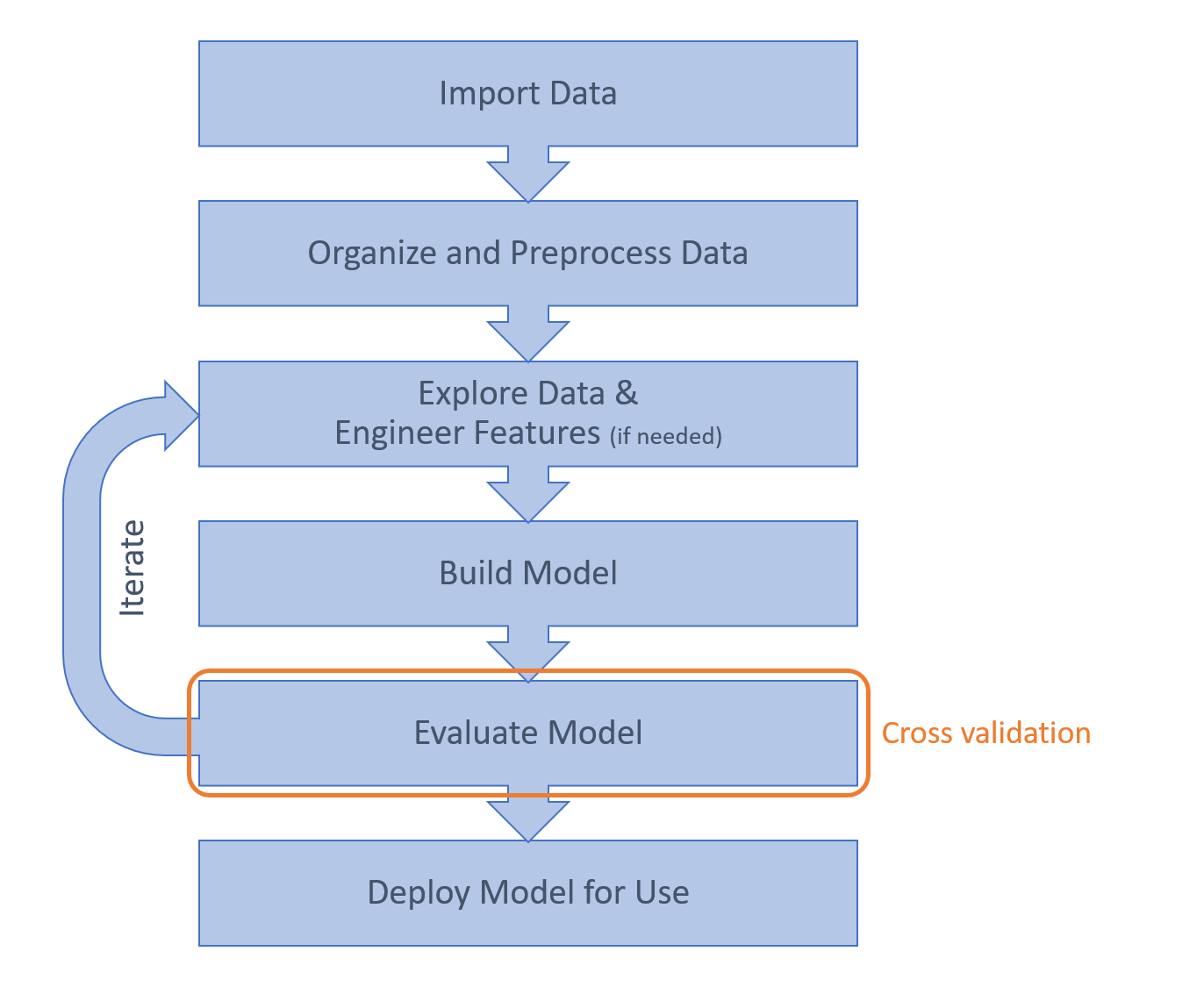
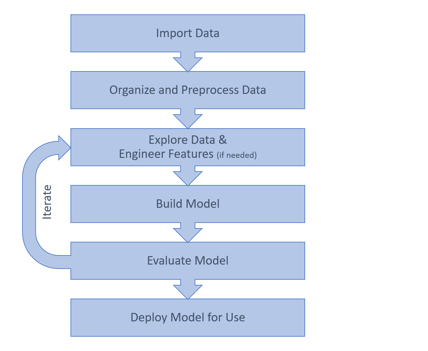
一、总体工作流程

二、分类工作流程

1.导入数据

letter = readtable("J.txt");

letter将成为一个类似excel的表格

通过点属性的方式，可以获取该列数据，下面利用plot绘制出来：

plot(letter.X,letter.Y)

 结果：

axis equal

可以通过该命令自动调节坐标系的比例：

2.处理数据 

letter = readtable("M.txt")
letter.X = 1.5*letter.X;
plot(letter.X,letter.Y)
axis equal

假如表中时间为ms级别，将表中的第一个时间作为起点做差，变成相对时间，最后除以1000，将时间单位变为秒。 

letter.Time = letter.Time - letter.Time(1)
letter.Time = letter.Time/1000

plot(letter.Time,letter.X)
plot(letter.Time,letter.Y)

 

 

这样做的好处就是将横坐标的数量级拉低。

3.提取特征

Calculating Features

 

What aspects of these letters could be used to distinguish a J from an M or a V? Instead of using the raw signals, the goal is to compute values that distill the entire signal into simple, useful units of information known as features.

• For the letters J and M, a simple feature might be the aspect ratio (the height of the letter relative to the width). A J is likely to be tall and narrow, whereas an M is likely to be more square.
• Compared to J and M, a V is quick to write, so the duration of the signal might also be a distinguishing feature.

letter = readtable("M.txt");
letter.X = letter.X*1.5;
letter.Time = (letter.Time - letter.Time(1))/1000
plot(letter.X,letter.Y)
axis equal

dur = letter.Time(end)%%取最后一个时间
aratio = range(letter.Y)/range(letter.X)

其中：

The range function returns the range of values in an array. That is, range(x) is equivalent to max(x)-min(x).

Viewing Features

load featuredata.mat
features

scatter(features.AspectRatio,features.Duration)

gscatter(features.AspectRatio,features.Duration,features.Character)

4.Build a Model

What is a Classification Model?

A classification model is a partitioning of the space of predictor variables into regions. Each region is assigned one of the output classes. In this simple example with two predictor variables, you can visualize these regions in the plane.

There is no single absolute “correct” way to partition the plane into the classes J, M, and V. Different classification algorithms result in different partitions.

下面开始训练模型：准备训练集和测试数据

load featuredata.mat

features

testdata

选用knn模型对训练集进行训练：

knnmodel = fitcknn(features,"Character")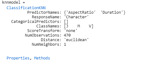

 

Making Predictions

Having built a model from the data, you can use it to classify new observations. This just requires calculating the features of the new observations and determining which region of the predictor space they are in.

predictions = predict(knnmodel,testdata)

The predict function determines the predicted class of new observations.

predClass = predict(model,newdata)

The inputs are the trained model and a table of observations, with the same predictor variables as were used to train the model. The output is a categorical array of the predicted class for each observation in newdata.

The file featuredata.mat contains a table testdata that has the same variables as features. However, the observations in testdata are not included in features.

Note that testdata contains observations for which the correct class is known (stored in the Character variable). This gives a way to test your model by comparing the classes predicted by the model with the true classes. The predict function will ignore the Character variable when making predictions from the model.

Algorithm Options

By default, fitcknn fits a kNN model with k = 1. That is, the model uses just the single closest known example to classify a given observation. This makes the model sensitive to any outliers in the training data, such as those highlighted in the image above. New observations near the outliers are likely to be misclassified.

You can make the model less sensitive to the specific observations in the training data by increasing the value of k (that is, use the most common class of several neighbors). Often this will improve the model's performance in general. However, how a model performs on any particular test set depends on the specific observations in that set. 

knnmodel = fitcknn(features,"Character","NumNeighbors",5)
predictions = predict(knnmodel,testdata)

最后，对比一下预测结果和测试样本： 

[predictions,testdata.Character]

6.Evaluate the Model

​load featuredata.mat
testdata
knnmodel = fitcknn(features,"Character","NumNeighbors",5);
predictions = predict(knnmodel,testdata)
iscorrect = predictions == testdata.Character
accuracy = sum(iscorrect)/numel(predictions)

 结果：

iswrong = predictions ~= testdata.Character
misclassrate = sum(iswrong)/numel(predictions)
[testdata.Character(iswrong) predictions(iswrong)]

 结果：

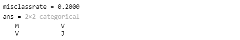
Accuracy and misclassification rate give a single value for the overall performance of the model, but it can be useful to see a more detailed breakdown of which classes the model confuses. A confusion matrix shows the number of observations for each combination of true and predicted class.

A confusion matrix is commonly visualized by shading the elements according to their value. Often the diagonal elements (the correct classifications) are shaded in one color and the other elements (the incorrect classifications) in another color. You can visualize a confusion matrix by using the confusionchart function.

confusionchart(ytrue,ypred);

where ytrue is a vector of the known classes and ypred is a vector of the predicted classes.

confusionchart(testdata.Character,predictions);

实例

load featuredata13letters.mat
features
testdata

 

gscatter(features.AspectRatio,features.Duration,features.Character)
xlim([0 10])

knnmodel = fitcknn(features,"Character","NumNeighbors",5);
predictions = predict(knnmodel,testdata);

misclass = sum(predictions ~= testdata.Character)/numel(predictions)
confusionchart(testdata.Character,predictions);

三、导入和预处理数据

1.Creating Datastores

Handwriting Sample Files

Samples of each letter were collected from many different volunteers. Some provided more than one sample of each letter. Each sample was saved in a separate file and all the files were stored in one folder. The file names have the form

user003_B_2.txt

This file would contain the second sample of the letter B written by the volunteer designated “user003”.

Use the datastore function to make a datastore to all files containing the letter M. These files have _M_ in their name and a .txt extension. Store the datastore in a variable called letterds

通过匹配文件名来打开一系列文件，*代表任意字符

letterds = datastore("*_M_*.txt")

You can use the read function to import the data from a file in the datastore.
data = read(ds);
Using the read function the first time will import the data from the first file. Using it a second time will import the data from the second file, and so on.

data = read(letterds)

plot(data.X,data.Y)

Calling the read function again imports the data from the next file in the datastore.

data = read(letterds)
plot(data.X,data.Y)

The readall function imports the data from all the files in the datastore into a single variable. 

data = readall(letterds)
plot(data.X,data.Y)

 2.Adding a Data Transformantion

Custom Preprocessing Functions

Typically you will want to apply a series of preprocessing operations to each sample of your raw data. The first step to automating this procedure is to make a custom function that applies your specific preprocessing operations. 

Transformed

Currently, you still need to call your function manually. To automate your data importing and preprocessing, you want your datastore to apply this function whenever the data is read. You can do this with a transformed datastore. The transform function takes a datastore and a function as inputs. It returns a new datastore as output. This transformed datastore applies the given function whenever it imports data.

Normalizing Data

The location of a letter is not important for classifying it. What matters is the shape. A common preprocessing step for many machine learning problems is to normalize the data.

Typical normalizations include shifting by the mean (so that the mean of the shifted data is 0) or shifting and scaling the data into a fixed range (such as [-1, 1]). In the case of the handwritten letters, shifting both the x and y data to have 0 mean will ensure that all the letters are centered around the same point.

letterds = datastore("*_M_*.txt");
data = read(letterds);
data = scale(data);
plot(data.X,data.Y)
axis equal
plot(data.Time,data.Y)
ylabel("Vertical position")
xlabel("Time")

function data = scale(data)
data.Time = (data.Time - data.Time(1))/1000;
data.X = 1.5*data.X;
data.X = data.X - mean(data.X,"omitnan");
data.Y = data.Y - mean(data.Y,"omitnan");
end

preprocds = transform(letterds,@scale)
data = readall(preprocds)
plot(data.Time,data.Y)

 

四、特征工程

Statistical Functions

Measures of Central Tendency

Function	Description
mean	Arithmetic mean
median	Median (middle) value
mode	Most frequent value
trimmean	Trimmed mean (mean, excluding outliers)
geomean	Geometric mean
harmean	Harmonic mean

Measures of Spread

Function	Description
range	Range of values (largest – smallest)
std	Standard deviation
var	Variance
mad	Mean absolute deviation
iqr	Interquartile range (75th percentile minus 25th percentile)

Measures of Shape

Function	Description
skewness	Skewness (third central moment)
kurtosis	Kurtosis (fourth central moment)
moment	Central moment of arbitrary order

1. Calculating Summary Statistic(Quantifying Letter Shapes)

Descriptive Statistics

The handwriting samples have all been shifted so they have zero mean in both horizontal and vertical position. What other statistics could provide information about the shape of the letters? Different letters will have different distributions of points. Statistical measures that describe the shape of these distributions could be useful features.

load sampleletters.mat
plot(b1.Time,b1.X)
hold on
plot(b2.Time,b2.X)
hold off
plot(b1.Time,b1.Y)
hold on
plot(b2.Time,b2.Y)
hold off

aratiob = range(b1.Y)/range(b1.X)
medxb = median(b1.X,"omitnan")
medyb = median(b1.Y,"omitnan")
devxb = mad(b1.X)
devyb = mad(b1.Y)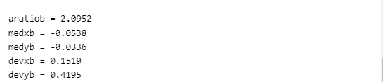

aratiov = range(v1.Y)/range(v1.X)
medxd = median(d1.X,"omitnan")
medyd = median(d1.Y,"omitnan")
devxm = mad(m1.X)
devym = mad(m1.Y)

plot(b1.X,b1.Y,b2.X,b2.Y)
axis([-1 1 -1 1])
axis equal
plot(d1.X,d1.Y,d2.X,d2.Y)
axis([-1 1 -1 1])
axis equal

2.Finding Peaks 

Local minima and maxima are often important features of a signal. The islocalmin and islocalmax functions take a signal as input and return a logical array the same length as the signal.
idx = islocalmin(x);
The value of idx is true whenever the corresponding value in the signal is a local minimum.

load sampleletters.mat
plot(m1.Time,m1.X)

idxmin = islocalmin(m1.X)
idxmax = islocalmax(m1.X)

plot(m1.Time,m1.X)
hold on
plot(m1.Time(idxmin),m1.X(idxmin),"o")
plot(m1.Time(idxmax),m1.X(idxmax),"s")
hold off

Local minima and maxima are defined by computing the prominence of each value in the signal. The prominence is a measure of how a value compares to the other values around it. You can obtain the prominence value of each point in a signal by obtaining a second output from islocalmin or islocalmax.

[idx,p] = islocalmin(x);

[idx,prom] = islocalmin(m1.X);
plot(m1.Time,prom)

 By default, islocalmin and islocalmax find points with any prominence value above 0. This means that a maximum is defined as any point that is larger than the two values on either side of it. For noisy signals you might want to consider only minima and maxima that have a prominence value above a given threshold.

idx = islocalmin(x,"MinProminence",threshvalue)

When choosing a threshold value, note that prominence values can range from 0 to range(x).

idxmin = islocalmin(m1.X,"MinProminence",0.1);
idxmax = islocalmax(m1.X,"MinProminence",0.1);
nnz(idxmin) 
sum(idxmin)

3.Computing Derivative 

Approximating Velocity

An important aspect of detecting letters written on a tablet is that there is useful information in the rhythm and flow of how the letters are written. To describe the shape of the signals through time, it can be useful to know the velocity of the pen, or, equivalently, the slope of the graph of position through time.

The raw data recorded from the tablet has only position (not velocity) through time, so velocity must be calculated from the raw data. With discrete data points, this means estimating the velocity by using a finite difference approximation v=Δx/Δt

load sampleletters.mat
plot(m2.Time,m2.X)
grid

dX = diff(m2.X);
dT = diff(m2.Time);
dXdT = dX./dT;
plot(m2.Time(1:end-1),dXdT)

maxdx = max(dXdT)
dYdT = diff(m2.Y)./dT;
maxdy = max(dYdT)

Due to limits on the resolution of the data collection procedure, the data contains some repeated values. If the position and the time are both repeated, then the differences are both 0, resulting in a derivative of 0/0 = NaN. However, if the position values are very slightly different, then the derivative will be Inf (nonzero divided by 0).

Note that max ignores NaN but not Inf because Inf is larger than any finite value. However, for this application, both NaN and Inf can be ignored, as they represent repeated data.

You can use the standardizeMissing function to convert a set of values to NaN (or the appropriate missing value for nonnumeric data types).

xclean = standardizeMissing(x,0);
Here, xclean will be the same as x (including any NaNs), but will have NaN wherever x had the value 0. 

dYdT = standardizeMissing(dYdT,Inf);
maxdy = max(dYdT)

Try calculating the derivatives of different sample letters. Note that a negative value divided by zero will result in -Inf. You can pass a vector of values to standardizeMissing to deal with multiple missing values at once.

xclean = standardizeMissing(x,[-Inf 0 Inf]);

dYdT = standardizeMissing(dYdT,[-Inf 0 Inf]);
maxdy = max(dYdT)

4.Calculating Correlations

Measuring Similarity

The pair of signals on the left have a significantly different shape to the pair of signals on the right. However, the relationship between the two signals in each pair is similar in both cases: in the blue regions, the upper signal is increasing while the lower signal is decreasing, and vice versa in the yellow regions. Correlation attempts to measure this similarity, regardless of the shape of the signal.

load sampleletters.mat
plot(v2.X,v2.Y,"o-")

For the first half of the letter V, the horizontal and vertical positions have a strong negative linear correlation: when the horizontal position increases, the vertical position decreases proportionally. Similarly, for the second half, the positions have a strong positive correlation: when the horizontal position increases, the vertical position also increases proportionally.
The corr function calculates the linear correlation between variables.

C = corr(x,y);

C = corr(v2.X,v2.Y)

结果：

C = NaN

Because both variables contain missing data, C is NaN. You can use the "Rows" option to specify how to avoid missing values.

C = corr(x,y,"Rows","complete");

C = corr(v2.X,v2.Y,"Rows","complete")

结果：

C = 0.6493

The correlation coefficient is always between -1 and +1.

• A coefficient of -1 indicates a perfect negative linear correlation
• A coefficient of +1 indicates a perfect positive linear correlation
• A coefficient of 0 indicates no linear correlation

In this case, there is only a moderate correlation because the calculation has been performed on the entire signal. It may be more informative to consider the two halves of the signal separately.

M = [v2.X(1:11) v2.Y(1:11) v2.X(12:22) v2.Y(12:22)]

To calculate the correlation between each pair of several variables, you can pass a matrix to the corr function, where each variable is a column of the matrix.

M = [x y z];
C = corr(M);

Cmat = corr(M,"Rows","complete")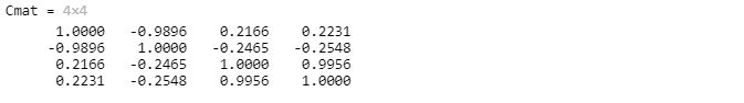

注意：进行列与列之间两两相关计算，由于X与Y的相关性和Y与X的相同，因此，该矩阵是一个对称矩阵。

The output Cmat is a 4-by-4 matrix of the coefficients of correlation between each pairwise combination of the columns of M. That is, Cmat(j,k) is the correlation of M(:,j) and M(:,k). The matrix is symmetric because the correlation between x and y is the same as the correlation between y and x. The diagonal elements are always equal to 1, because a variable is always perfectly correlated with itself.

5.Automating Feature Extraction

Custom Preprocessing Functions

Once you have determined the features you want to extract, you will need to apply the appropriate calculations to every sample in your data set. The first step to automating this procedure is to make a custom function that takes the data as input and returns an array of features as output.

Creating a Feature Extraction Function

Currently the script calculates six features for a given letter (stored in the variable letter). The six features are stored in six separate variables.
You can use the table function to combine separate variables into a table.

T = table(x,y,z);

load sampleletters.mat
letter = b1;

aratio = range(letter.Y)/range(letter.X)
idxmin = islocalmin(letter.X,"MinProminence",0.1);
numXmin = nnz(idxmin)
idxmax = islocalmax(letter.Y,"MinProminence",0.1);
numYmax = nnz(idxmax)
dT = diff(letter.Time);
dXdT = diff(letter.X)./dT;
dYdT = diff(letter.Y)./dT;
avgdX = mean(dXdT,"omitnan")
avgdY = mean(dYdT,"omitnan")
corrXY = corr(letter.X,letter.Y,"rows","complete")

featurenames = ["AspectRatio","NumMinX","NumMinY","AvgU","AvgV","CorrXY"];

 By default, the table constructed with the table function has default variable names. To make a table with more useful names, use the 'VariableNames' option.

T = table(x,y,z,'VariableNames',["X","Y","Z"]);

Typically you can use either single or double quotes to specify option names. However, because strings can represent data for your table, you need to use single quotes when specifying the 'VariableNames' option.

feat = table(aratio,numXmin,numYmax,avgdX,avgdY,corrXY)

feat = table(aratio,numXmin,numYmax,avgdX,avgdY,corrXY,'VariableNames',featurenames)

At the end of the script, add a local function called extract that takes a single variable, letter, as input and returns a table of features, feat, as output. Copy the code from the beginning of the script and from task 2 to make the body of the function. Test your function by calling it with b2 as input. Store the result in a variable called featB2. 

featB2 = extract(b2)


function feat = extract(letter)
aratio = range(letter.Y)/range(letter.X);
idxmin = islocalmin(letter.X,"MinProminence",0.1);
numXmin = nnz(idxmin);
idxmax = islocalmax(letter.Y,"MinProminence",0.1);
numYmax = nnz(idxmax);
dT = diff(letter.Time);
dXdT = diff(letter.X)./dT;
dYdT = diff(letter.Y)./dT;
avgdX = mean(dXdT,"omitnan");
avgdY = mean(dYdT,"omitnan");
corrXY = corr(letter.X,letter.Y,"rows","complete");

featurenames = ["AspectRatio","NumMinX","NumMinY","AvgU","AvgV","CorrXY"];

feat = table(aratio,numXmin,numYmax,avgdX,avgdY,corrXY,'VariableNames',featurenames);
end

Extracting Features from Multiple Data Files

Transformed Datastores

 To automate your feature extraction, you want your datastore to apply your extraction function whenever the data is read. As with preprocessing, you can do this with a transformed datastore.

From the raw data, you will typically need to apply both preprocessing and feature extraction functions. You can apply the transform function repeatedly to add any number of transformations to the datastore to the raw data.

The script currently applies the scale function to the files in the datastore letterds. The transformed datastore is stored in the variable preprocds.

letterds = datastore("*.txt");
preprocds = transform(letterds,@scale)

featds = transform(preprocds,@extract)

function data = scale(data)
% Normalize time [0 1]
data.Time = (data.Time - data.Time(1))/(data.Time(end) - data.Time(1));
% Fix aspect ratio
data.X = 1.5*data.X;
% Center X & Y at (0,0)
data.X = data.X - mean(data.X,"omitnan");
data.Y = data.Y - mean(data.Y,"omitnan");
% Scale to have bounding box area = 1
scl = 1/sqrt(range(data.X)*range(data.Y));
data.X = scl*data.X;
data.Y = scl*data.Y;
end

function feat = extract(letter)
% Aspect ratio
aratio = range(letter.Y)/range(letter.X);
% Local max/mins
idxmin = islocalmin(letter.X,"MinProminence",0.1);
numXmin = nnz(idxmin);
idxmax = islocalmax(letter.Y,"MinProminence",0.1);
numYmax = nnz(idxmax);
% Velocity
dT = diff(letter.Time);
dXdT = diff(letter.X)./dT;
dYdT = diff(letter.Y)./dT;
avgdX = mean(dXdT,"omitnan");
avgdY = mean(dYdT,"omitnan");
% Correlation
corrXY = corr(letter.X,letter.Y,"rows","complete");
% Put it all together into a table
featurenames = ["AspectRatio","NumMinX","NumMinY","AvgU","AvgV","CorrXY"];
feat = table(aratio,numXmin,numYmax,avgdX,avgdY,corrXY,'VariableNames',featurenames);
end

 Use the readall function to read, preprocess, and extract features from all the data files. Store the result in a variable called data.
There are 12 files and the extract function calculates six features for each. Hence, data should be a 12-by-6 table.
Visualize the imported data by making a scatter plot of AspectRatio on the x-axis and CorrXY on the y-axis.

data = readall(featds)
scatter(data.AspectRatio,data.CorrXY)

 The letters that the data represents are given in the data file names, which are of the form usernnn_X_n.txt. Note that the letter name appears between underscore characters (_X_).
You can use the extractBetween function to extract text that occurs between given strings.

extractedtxt = extractBetween(txt,"abc","xyz")

If txt is the string array ["hello abc 123 xyz","abcxyz","xyzabchelloxyzabc"], then extractedtxt will be [" 123 ","","hello"].

knownchar = extractBetween(letterds.Files,"_","_")

For classification problems, you typically want to represent the known label as a categorical variable. You can use the categorical function to convert an array to categorical type.
xcat = categorical(x)
By default, the unique values in x will be used to define the set of categories.

knownchar = categorical(knownchar)

It is convenient to have the known classes associated with the training data. Recall that you can create new variables in a table by assigning to a variable using dot notation.

T.newvar = workspacevar

data.Character = knownchar
gscatter(data.AspectRatio,data.CorrXY,data.Character)

五、分类模型

1.Training a Model

Handwriting Features

The MAT-file letterdata.mat contains the table traindata which represents feature data for 2906 samples of individual letters. There are 25 features, including statistical measures, correlations, and maxima/minima for the position, velocity, and pressure of the pen.

load letterdata.mat
traindata

histogram(traindata.Character)

A boxplot is a simple way to visualize multiple distributions.
boxplot(x,c)
This creates a plot where the boxes represent the distribution of the values of x for each of the classes in c. If the values of x are typically significantly different for one class than another, then x is a feature that can distinguish between those classes. The more features you have that can distinguish different classes, the more likely you are to be able to build an accurate classification model from the full data set. 

boxplot(traindata.MADX,traindata.Character)

 Use the command classificationLearner to open the Classification Learner app.

• Select traindata as the data to use.
• The app should correctly detect Character as the response variable to predict.
• Choose the default validation option.
• Select a model and click the Train button.

Try a few of the standard models with default options. See if you can achieve at least 80% accuracy.

Note that SVMs work on binary classification problems (i.e. where there are only two classes). To make SVMs work on this problem, the app is fitting many SVMs. These models will therefore be slow to train.

Similarly, ensemble methods work by fitting multiple models. These will also be slow to train.

2.Making Predictions

The MAT-file letterdata.mat contains traindata, the table of data used to train the model knnmodel. It also contains testdata which is a table of data (with the same features as traindata) that the model has never seen before.
Recall that you can use the predict function to obtain a model's predictions for new data.

preds = predict(model,newdata)

load letterdata.mat
traindata
knnmodel = fitcknn(traindata,"Character","NumNeighbors",5,"Standardize",true,"DistanceWeight","squaredinverse");
testdata

predLetter = predict(knnmodel,testdata)

misclassrate = sum(predLetter ~= testdata.Character)/numel(predLetter)

The response classes are not always equally distributed in either the training or test data. Loss is a fairer measure of misclassification that incorporates the probability of each class (based on the distribution in the data).

loss(model,testdata)

testloss = loss(knnmodel,testdata)

3.Investigating Misclassifications（Identifying Common Misclassifications）

The Confusion Matrix

For any response class X, you can divide a machine learning model's predictions into four groups:

• True positives (green) – predicted to be X and was actually X
• True negatives (blue) – predicted to be not X and was actually not X
• False positives (yellow) – predicted to be X but was actually not X
• False negatives (orange) – predicted to be not X but was actually X

 False Negatives

With 26 letters, you will need to enlarge the confusion chart to make the values visible. If you open the plot in a separate figure, you can resize it as large as you like.

The row summary shows the false negative rate for each class. This shows which letters the kNN model has the most difficulty identifying (i.e., the letters the model most often thinks are som

 This model has particular difficulty with the letter U, most often mistaking it for M, N, or V.

Some confusions seem reasonable, such as U/V or H/N. Others are more surprising, such as U/K. Having identified misclassifications of interest, you will probably want to look at some the specific data samples to understand what is causing the misclassification.

Identifying Common Misclassifications

When making a confusion chart, you can add information about the false negative and false positive rate for each class by adding row or column summaries, respectively.

confusionchart(...,"RowSummary","row-normalized");

load letterdata.mat
load predmodel.mat
testdata
predLetter
confusionchart(testdata.Character,predLetter);

confusionchart(testdata.Character,predLetter,"RowSummary","row-normalized");

Recall that the Files property of a datastore contains the file names of the original data. Hence, when you import the data and extract the features, you can keep a record of which data file is associated with each observation. The string array testfiles contains the file names for the test data. 

Use the logical array falseneg as an index into testfiles to determine the file names of the observations that were incorrectly classified as the letter U. Store the result in a variable called fnfiles.

Similarly, use falseneg as an index into predLetter to determine the associated predicted letters. Store the result in a variable called fnpred.

falseneg = (testdata.Character == "U") & (predLetter ~= "U");

fnfiles = testfiles(falseneg)
fnpred = predLetter(falseneg)

 Use the readtable function to import the data in the fourth element of fnfiles into a table called badU. Visualize the letter by plotting Y against X.

badU = readtable(fnfiles(4));
plot(badU.X,badU.Y)
title("Prediction: "+string(fnpred(4)))

4.Investigating Misclassifications（Investigating Features）

load letterdata.mat
load predmodel.mat
traindata
testdata
predLetter

idx = (traindata.Character == "N") | (traindata.Character == "U");
UorN = traindata(idx,:)

idx = (testdata.Character == "U") & (predLetter ~= "U");
fnU = testdata(idx,:)

 Categorical variables maintain the full list of possible classes, even when only a subset are present in the data. When examining a subset, it can be useful to redefine the set of possible classes to only those that are in the data. The removecats function removes unused categories.

cmin = removecats(cfull)

UorN.Character = removecats(UorN.Character);

 You can use curly braces ({ }) to extract data from a table into an array of a single type.
datamatrix = datatable{1:10,4:6}
This extracts the first 10 elements of variables 4, 5, and 6. If these variables are numeric, datamatrix will be a 10-by-3 double array.

UorNfeat = UorN{:,1:end-1};
fnUfeat = fnU{:,1:end-1};

A parallel coordinates plot shows the value of the features (or “coordinates”) for each observation as a line.
parallelcoords(data)

To compare the feature values of different classes, use the "Group" option.
parallelcoords(data,"Group",classes)

parallelcoords(UorNfeat,"Group",UorN.Character)

Because a parallel coordinates plot is just a line plot, you can add individual observations using the regular plot function.

hold on
plot(fnUfeat(4,:),"k")
hold off

Use the zoom tool to explore the plot. Note that N and U have similar values for many features. Are there any features that help distinguish these letters from each other? A kNN model uses the distance between observations, where the distance is calculated over all the features. Does this explain why N and U are hard to distinguish, even if there are some features that separate them?

When plotting multiple observations by groups, it can be helpful to view the median and a range for each group, rather than every individual observation. You can use the "Quantile" option to do this.

parallelcoords(...,"Quantile",0.2)

parallelcoords(UorNfeat,"Group",UorN.Character,"Quantile",0.2)

5. Improving the Model

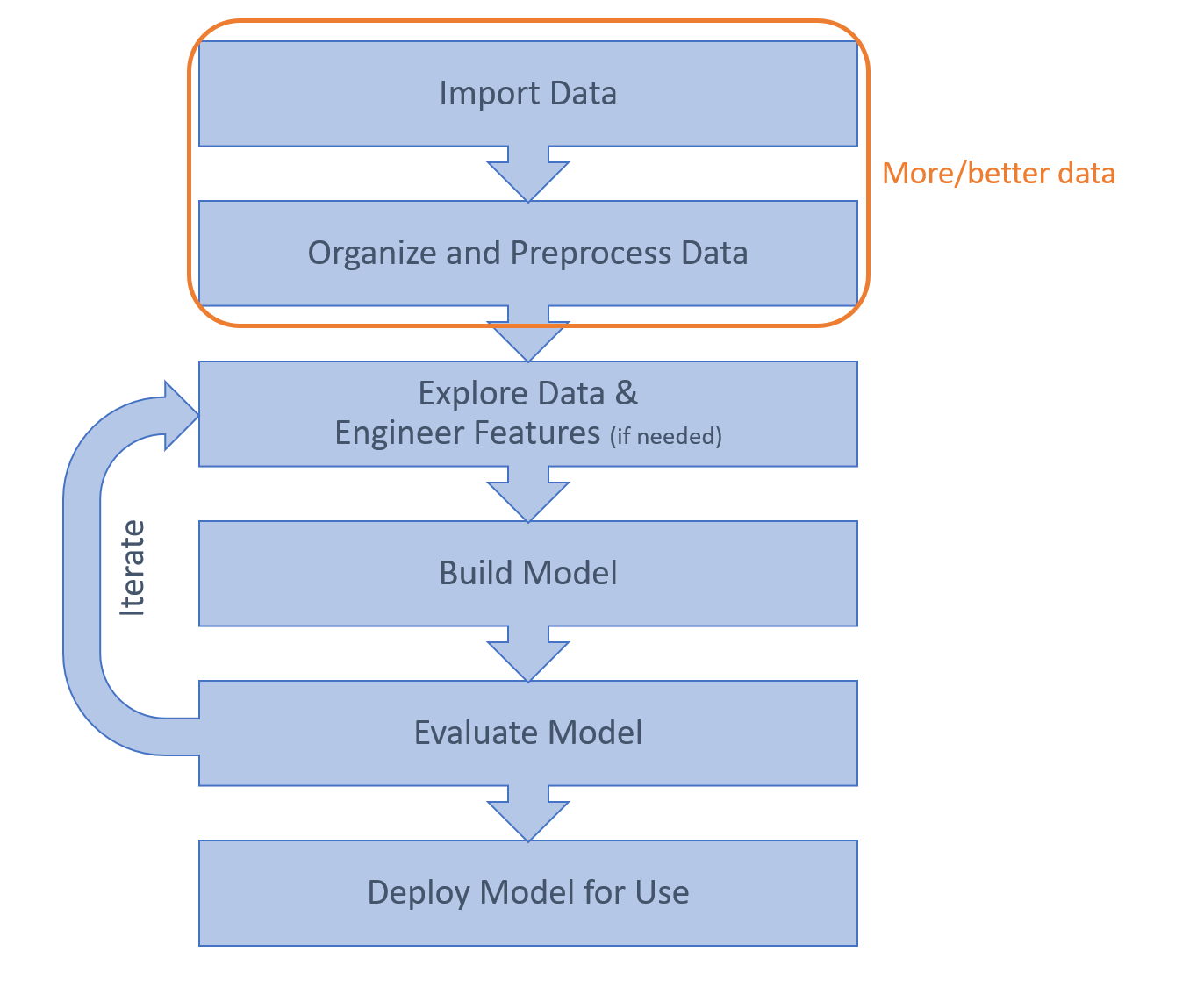
Even if your model works well, you will typically want to look for improvements before deploying it for use. Theoretically, you could try to improve your results at any part of the workflow. However, collecting data is typically the most difficult step of the process, which means you often have to work with the data you have.

If you have the option of collecting more data, you can use the insights you have gained so far to inform what new data you need to collect.

In the handwriting example, volunteers were instructed only to write lower-case letters “naturally”. Investigating the data set reveals that there are often discrete groups within a particular letter, such as a block-letter style and a cursive style. This means that two quite different sets of features can represent the same letter.

One way to improve the model would be treat these variants as separate classes. However, this would mean having many more than 26 classes. To train such a model, you would need to collect more samples, instruct the volunteers to write both block and cursive style, and label the collected data accordingly.

 

If you have the option of collecting more data, you can use the insights you have gained so far to inform what new data you need to collect.

In the handwriting example, volunteers were instructed only to write lower-case letters “naturally”. Investigating the data set reveals that there are often discrete groups within a particular letter, such as a block-letter style and a cursive style. This means that two quite different sets of features can represent the same letter.

One way to improve the model would be treat these variants as separate classes. However, this would mean having many more than 26 classes. To train such a model, you would need to collect more samples, instruct the volunteers to write both block and cursive style, and label the collected data accordingly.

Low accuracy in both your training and testing sets is an indication that your features do not provide enough information to distinguish the different classes. In particular, you might want to look at the data for classes that are frequently confused, to see if there are characteristics that you can capture as new features.

However, too many features can also be a problem. Redundant or irrelevant features often lead to low accuracy and increase the chance of overfitting – when your model is learning the details of the training rather than the broad patterns. A common sign of overfitting is that your model performs well on the training set but not on new data. You can use a feature selection technique to find and remove features that do not significantly add to the performance of your model.

You can also use feature transformation to perform a change of coordinates on your features. With a technique such as Principal Component Analysis (PCA), the transformed features are chosen to minimize redundancy and ordered by how much information they contain.

Low accuracy in both your training and testing sets is an indication that your features do not provide enough information to distinguish the different classes. In particular, you might want to look at the data for classes that are frequently confused, to see if there are characteristics that you can capture as new features.

However, too many features can also be a problem. Redundant or irrelevant features often lead to low accuracy and increase the chance of overfitting – when your model is learning the details of the training rather than the broad patterns. A common sign of overfitting is that your model performs well on the training set but not on new data. You can use a feature selection technique to find and remove features that do not significantly add to the performance of your model.

You can also use feature transformation to perform a change of coordinates on your features. With a technique such as Principal Component Analysis (PCA), the transformed features are chosen to minimize redundancy and ordered by how much information they contain.

The Classification Learner app provides an easy way to experiment with different models. You can also try different options. For example, for kNN models, you can vary the number of neighbors, the weighting of the neighbors based on distance, and the way that distance is defined.

Some classification methods are highly sensitive to the training data, which means you might get very different predictions from different models trained on different subsets of the data. This can be harnessed as a strength by making an ensemble – training a large number of these so-called weak learners on different permutations of the training data and using the distribution of individual predictions to make the final prediction.

For the handwriting example, some pairs of letters (such as N and V) have many similar features and are distinguished by only one or two key features. This means that a distance-based method such as kNN may have difficulty with these pairs. An alternative approach is to use an ensemble approach known as Error-Correcting Output Coding (ECOC) which use multiple models to distinguish between different binary pairs of classes. Hence, one model can distinguish between N and V, while another can distinguish between N and E, and another between E and V, and so on.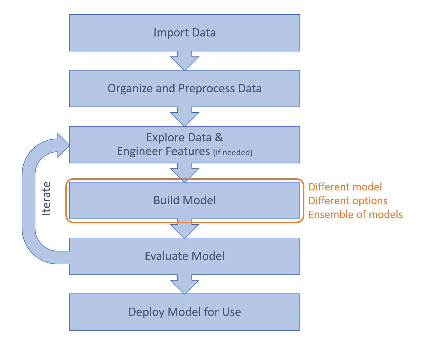

When trying to evaluate different models, it is important to have an accurate measure of a model's performance. The simplest, and computationally cheapest, way to do validation is holdout – randomly divide your data into a training set and a testing set. This works for large data sets. However, for many problems, holdout validation can result in the test accuracy being dependent on the specific choice of test data.

You can use k-fold cross-validation to get a more accurate estimate of performance. In this approach, multiple models are trained and tested, each on a different division of the data. The reported accuracy is the average from the different models.

Accuracy is only one simple measure of the model's performance. It is also important to consider the confusion matrix, false negative rates, and false positive rates. Furthermore, the practical impact of a false negative may be significantly different to that of a false positive. For example, a false positive medical diagnosis may cause stress and expense, but a false negative could be fatal. In these cases, you can incorporate a cost matrix into the calculation of a model's loss.