测试题:参考博文
作业1:实现卷积神经网络
1. 导入一些包
import numpy as np
import h5py
import matplotlib.pyplot as plt

%matplotlib inline
plt.rcParams['figure.figsize'] = (5.0, 4.0) # set default size of plots
plt.rcParams['image.interpolation'] = 'nearest'
plt.rcParams['image.cmap'] = 'gray'

%load_ext autoreload
%autoreload 2

np.random.seed(1)
2. 模型框架
3. 卷积神经网络

卷积神经网络会将输入转化为一个维度大小不一样的输出
3.1 Zero-Padding
0 padding 会在图片周围填充 0 元素(下图 p = 2 p=2 p=2 )

padding 的好处:
- 减少深层网络里,图片尺寸衰减问题
- 保留更多的图片边缘的信息
# 给第2、4个维度 padding 1层,3层像素
a = np.pad(a, ((0,0), (1,1), (0,0), (3,3), (0,0)), 'constant', constant_values = (..,..))
# GRADED FUNCTION: zero_pad

def zero_pad(X, pad):
    """
    Pad with zeros all images of the dataset X. The padding is applied to the height and width of an image,
    as illustrated in Figure 1.

    Argument:
    X -- python numpy array of shape (m, n_H, n_W, n_C) representing a batch of m images
    pad -- integer, amount of padding around each image on vertical and horizontal dimensions

    Returns:
    X_pad -- padded image of shape (m, n_H + 2*pad, n_W + 2*pad, n_C)
    """

    ### START CODE HERE ### (≈ 1 line)
    X_pad = np.pad(X, ((0,0), # 样本
                       (pad,pad), # 高
                       (pad,pad), # 宽
                       (0,0)),# 通道
                   'constant', constant_values=(0))
    ### END CODE HERE ###

    return X_pad

3.2 单步卷积

# GRADED FUNCTION: conv_single_step

def conv_single_step(a_slice_prev, W, b):
    """
    Apply one filter defined by parameters W on a single slice (a_slice_prev) of the output activation
    of the previous layer.

    Arguments:
    a_slice_prev -- slice of input data of shape (f, f, n_C_prev)
    W -- Weight parameters contained in a window - matrix of shape (f, f, n_C_prev)
    b -- Bias parameters contained in a window - matrix of shape (1, 1, 1)

    Returns:
    Z -- a scalar value, result of convolving the sliding window (W, b) on a slice x of the input data
    """

    ### START CODE HERE ### (≈ 2 lines of code)
    # Element-wise product between a_slice and W. Do not add the bias yet.
    s = a_slice_prev*W
    # Sum over all entries of the volume s.
    Z = np.sum(s)
    # Add bias b to Z. Cast b to a float() so that Z results in a scalar value.
    Z = Z + float(b)
    ### END CODE HERE ###

    return Z
3.3 卷积神经网络 - 前向传播


n H = ⌊ n H p r e v − f + 2 × p a d s t r i d e ⌋ + 1 n_H = \lfloor \frac{n_{H_{prev}} - f + 2 \times pad}{stride} \rfloor +1 nH=⌊stridenHprev−f+2×pad⌋+1
n W = ⌊ n W p r e v − f + 2 × p a d s t r i d e ⌋ + 1 n_W = \lfloor \frac{n_{W_{prev}} - f + 2 \times pad}{stride} \rfloor +1 nW=⌊stridenWprev−f+2×pad⌋+1
n C = 卷积过滤器数量 n_C = \text{卷积过滤器数量} nC=卷积过滤器数量
# GRADED FUNCTION: conv_forward

def conv_forward(A_prev, W, b, hparameters):
    """
    Implements the forward propagation for a convolution function

    Arguments:
    A_prev -- output activations of the previous layer, numpy array of shape (m, n_H_prev, n_W_prev, n_C_prev)
    W -- Weights, numpy array of shape (f, f, n_C_prev, n_C)
    b -- Biases, numpy array of shape (1, 1, 1, n_C)
    hparameters -- python dictionary containing "stride" and "pad"

    Returns:
    Z -- conv output, numpy array of shape (m, n_H, n_W, n_C)
    cache -- cache of values needed for the conv_backward() function
    """

    ### START CODE HERE ###
    # Retrieve dimensions from A_prev's shape (≈1 line)
    (m, n_H_prev, n_W_prev, n_C_prev) = A_prev.shape

    # Retrieve dimensions from W's shape (≈1 line)
    (f, f, n_C_prev, n_C) = W.shape

    # Retrieve information from "hparameters" (≈2 lines)
    stride = hparameters['stride']
    pad = hparameters['pad']

    # Compute the dimensions of the CONV output volume using the formula given above.
    # Hint: use int() to floor. (≈2 lines)
    n_H = (n_H_prev-f+2*pad)//stride + 1
    n_W = (n_W_prev-f+2*pad)//stride + 1

    # Initialize the output volume Z with zeros. (≈1 line)
    Z = np.zeros((m, n_H, n_W, n_C))

    # Create A_prev_pad by padding A_prev
    A_prev_pad = zero_pad(A_prev, pad)

    for i in range(m):                      # loop over the batch of training examples
        a_prev_pad = A_prev_pad[i, :]      # Select ith training example's padded activation
        for h in range(n_H):               # loop over vertical axis of the output volume
            for w in range(n_W):          # loop over horizontal axis of the output volume
                for c in range(n_C):      # loop over channels (= #filters) of the output volume

                    # Find the corners of the current "slice" (≈4 lines)
                    vert_start = h*stride
                    vert_end = vert_start + f
                    horiz_start = w*stride
                    horiz_end = horiz_start + f

                    # Use the corners to define the (3D) slice of a_prev_pad (See Hint above the cell). (≈1 line)
                    a_slice_prev = a_prev_pad[vert_start:vert_end, horiz_start:horiz_end, :]

                    # Convolve the (3D) slice with the correct filter W and bias b, to get back one output neuron. (≈1 line)
                    Z[i, h, w, c] = np.sum(conv_single_step(a_slice_prev, W[:,:,:,c], b[:,:,:,c]))

    ### END CODE HERE ###

    # Making sure your output shape is correct
    assert(Z.shape == (m, n_H, n_W, n_C))

    # Save information in "cache" for the backprop
    cache = (A_prev, W, b, hparameters)

    return Z, cache
4. 池化层
池化层不改变通道数量,下面公式没有padding, p = 0
n H = ⌊ n H p r e v − f s t r i d e ⌋ + 1 n_H = \lfloor \frac{n_{H_{prev}} - f}{stride} \rfloor +1 nH=⌊stridenHprev−f⌋+1
n W = ⌊ n W p r e v − f s t r i d e ⌋ + 1 n_W = \lfloor \frac{n_{W_{prev}} - f}{stride} \rfloor +1 nW=⌊stridenWprev−f⌋+1
n C = n C p r e v n_C = n_{C_{prev}} nC=nCprev
# GRADED FUNCTION: pool_forward

def pool_forward(A_prev, hparameters, mode = "max"):
    """
    Implements the forward pass of the pooling layer

    Arguments:
    A_prev -- Input data, numpy array of shape (m, n_H_prev, n_W_prev, n_C_prev)
    hparameters -- python dictionary containing "f" and "stride"
    mode -- the pooling mode you would like to use, defined as a string ("max" or "average")

    Returns:
    A -- output of the pool layer, a numpy array of shape (m, n_H, n_W, n_C)
    cache -- cache used in the backward pass of the pooling layer, contains the input and hparameters
    """

    # Retrieve dimensions from the input shape
    (m, n_H_prev, n_W_prev, n_C_prev) = A_prev.shape

    # Retrieve hyperparameters from "hparameters"
    f = hparameters["f"]
    stride = hparameters["stride"]

    # Define the dimensions of the output
    n_H = 1 + (n_H_prev - f) // stride
    n_W = 1 + (n_W_prev - f) // stride
    n_C = n_C_prev

    # Initialize output matrix A
    A = np.zeros((m, n_H, n_W, n_C))

    ### START CODE HERE ###
    for i in range(m):                         # loop over the training examples
        for h in range(n_H):                     # loop on the vertical axis of the output volume
            for w in range(n_W):                 # loop on the horizontal axis of the output volume
                for c in range (n_C):            # loop over the channels of the output volume

                    # Find the corners of the current "slice" (≈4 lines)
                    vert_start = h*stride
                    vert_end = vert_start + f
                    horiz_start = w*stride
                    horiz_end = horiz_start + f

                    # Use the corners to define the current slice on the ith training example of A_prev, channel c. (≈1 line)
                    a_prev_slice = A_prev[i, vert_start:vert_end, horiz_start:horiz_end, c]

                    # Compute the pooling operation on the slice. Use an if statment to differentiate the modes. Use np.max/np.mean.
                    if mode == "max":
                        A[i, h, w, c] = np.max(a_prev_slice)
                    elif mode == "average":
                        A[i, h, w, c] = np.mean(a_prev_slice)

    ### END CODE HERE ###

    # Store the input and hparameters in "cache" for pool_backward()
    cache = (A_prev, hparameters)

    # Making sure your output shape is correct
    assert(A.shape == (m, n_H, n_W, n_C))

    return A, cache
5. 卷积神经网络 - 反向传播
现代机器学习框架一般都会自动帮你实现反向传播,下面再过一遍
5.1 卷积层反向传播
5.1.1 计算 dA
d A + = ∑ h = 0 n H ∑ w = 0 n W W c × d Z h w dA += \sum _{h=0} ^{n_H} \sum_{w=0} ^{n_W} W_c \times dZ_{hw} dA+=h=0∑nHw=0∑nWWc×dZhw
- W c W_c Wc 是一个过滤器, d Z h w dZ_{hw} dZhw 是输出的卷积层 Z Z Z 的(h,w)位置的梯度
代码:
da_prev_pad[vert_start:vert_end, horiz_start:horiz_end, :] += W[:,:,:,c] * dZ[i, h, w, c]
5.1.2 计算 dW
d W c + = ∑ h = 0 n H ∑ w = 0 n W a s l i c e × d Z h w dW_c += \sum _{h=0} ^{n_H} \sum_{w=0} ^ {n_W} a_{slice} \times dZ_{hw} dWc+=h=0∑nHw=0∑nWaslice×dZhw
代码:
dW[:,:,:,c] += a_slice * dZ[i, h, w, c]
5.1.3 计算 db
d b = ∑ h ∑ w d Z h w db = \sum_h \sum_w dZ_{hw} db=h∑w∑dZhw
代码:
db[:,:,:,c] += dZ[i, h, w, c]
def conv_backward(dZ, cache):
    """
    Implement the backward propagation for a convolution function

    Arguments:
    dZ -- gradient of the cost with respect to the output of the conv layer (Z), numpy array of shape (m, n_H, n_W, n_C)
    cache -- cache of values needed for the conv_backward(), output of conv_forward()

    Returns:
    dA_prev -- gradient of the cost with respect to the input of the conv layer (A_prev),
               numpy array of shape (m, n_H_prev, n_W_prev, n_C_prev)
    dW -- gradient of the cost with respect to the weights of the conv layer (W)
          numpy array of shape (f, f, n_C_prev, n_C)
    db -- gradient of the cost with respect to the biases of the conv layer (b)
          numpy array of shape (1, 1, 1, n_C)
    """

    ### START CODE HERE ###
    # Retrieve information from "cache"
    (A_prev, W, b, hparameters) = cache

    # Retrieve dimensions from A_prev's shape
    (m, n_H_prev, n_W_prev, n_C_prev) = A_prev.shape

    # Retrieve dimensions from W's shape
    (f, f, n_C_prev, n_C) = W.shape

    # Retrieve information from "hparameters"
    stride = hparameters['stride']
    pad = hparameters['pad']

    # Retrieve dimensions from dZ's shape
    (m, n_H, n_W, n_C) = dZ.shape

    # Initialize dA_prev, dW, db with the correct shapes
    dA_prev = np.zeros(A_prev.shape)
    dW = np.zeros(W.shape)
    db = np.zeros((1, 1, 1, n_C))

    # Pad A_prev and dA_prev, 添加周围pad像素
    A_prev_pad = zero_pad(A_prev, pad)
    dA_prev_pad = zero_pad(dA_prev, pad)

    for i in range(m):                       # loop over the training examples

        # select ith training example from A_prev_pad and dA_prev_pad
        a_prev_pad = A_prev_pad[i]
        da_prev_pad = dA_prev_pad[i]

        for h in range(n_H):                   # loop over vertical axis of the output volume
            for w in range(n_W):               # loop over horizontal axis of the output volume
                for c in range(n_C):           # loop over the channels of the output volume

                    # Find the corners of the current "slice"
                    vert_start = h*stride
                    vert_end = vert_start + f
                    horiz_start = w*stride
                    horiz_end = horiz_start + f

                    # Use the corners to define the slice from a_prev_pad
                    a_slice = a_prev_pad[vert_start:vert_end, horiz_start:horiz_end, :]

                    # Update gradients for the window and the filter's parameters using the code formulas given above
                    da_prev_pad[vert_start:vert_end, horiz_start:horiz_end, :] += W[:,:,:,c]*dZ[i,h,w,c]
                    dW[:,:,:,c] += a_slice*dZ[i,h,w,c]
                    db[:,:,:,c] += dZ[i,h,w,c]

        # Set the ith training example's dA_prev to the unpaded da_prev_pad (Hint: use X[pad:-pad, pad:-pad, :])
        dA_prev[i, :, :, :] = da_prev_pad[pad:-pad, pad:-pad, :]
    ### END CODE HERE ###

    # Making sure your output shape is correct
    assert(dA_prev.shape == (m, n_H_prev, n_W_prev, n_C_prev))

    return dA_prev, dW, db
5.2 池化层 - 反向传播
池化层没有参数需要更新
5.2.1 最大池化 - 反向传播
先建立一个辅助函数create_mask_from_window():
X = [ 1 3 4 2 ] → M = [ 0 0 1 0 ] X = \begin{bmatrix} 1 && 3 \\ 4 && 2 \end{bmatrix} \quad \rightarrow \quad M =\begin{bmatrix} 0 && 0 \\ 1 && 0 \end{bmatrix} X=[1432]→M=[0100]
可以使用 x = np.max(X), A = (X == x)
def create_mask_from_window(x):
    """
    Creates a mask from an input matrix x, to identify the max entry of x.

    Arguments:
    x -- Array of shape (f, f)

    Returns:
    mask -- Array of the same shape as window,
        contains a True at the position corresponding to the max entry of x.
    """

    ### START CODE HERE ### (≈1 line)
    mask = (x == np.max(x))
    ### END CODE HERE ###

    return mask
5.2.2 平均池化 - 反向传播
平均池化,输入的每个元素是一样的重要对于输出,反向传播时:
d Z = 1 → d Z = [ 1 / 4 1 / 4 1 / 4 1 / 4 ] dZ = 1 \quad \rightarrow \quad dZ =\begin{bmatrix} 1/4 && 1/4 \\ 1/4 && 1/4 \end{bmatrix} dZ=1→dZ=[1/41/41/41/4]
def distribute_value(dz, shape):
    """
    Distributes the input value in the matrix of dimension shape

    Arguments:
    dz -- input scalar
    shape -- the shape (n_H, n_W) of the output matrix for which we want to distribute the value of dz

    Returns:
    a -- Array of size (n_H, n_W) for which we distributed the value of dz
    """

    ### START CODE HERE ###
    # Retrieve dimensions from shape (≈1 line)
    (n_H, n_W) = shape

    # Compute the value to distribute on the matrix (≈1 line)
    average = dz/(n_H*n_W)

    # Create a matrix where every entry is the "average" value (≈1 line)
    a =np.ones((n_H, n_W))*average
    ### END CODE HERE ###

    return a
5.2.3 组合在一起 - 反向池化
def pool_backward(dA, cache, mode = "max"):
    """
    Implements the backward pass of the pooling layer

    Arguments:
    dA -- gradient of cost with respect to the output of the pooling layer, same shape as A
    cache -- cache output from the forward pass of the pooling layer, contains the layer's input and hparameters
    mode -- the pooling mode you would like to use, defined as a string ("max" or "average")

    Returns:
    dA_prev -- gradient of cost with respect to the input of the pooling layer, same shape as A_prev
    """

    ### START CODE HERE ###

    # Retrieve information from cache (≈1 line)
    (A_prev, hparameters) = cache

    # Retrieve hyperparameters from "hparameters" (≈2 lines)
    stride = hparameters['stride']
    f = hparameters['f']

    # Retrieve dimensions from A_prev's shape and dA's shape (≈2 lines)
    m, n_H_prev, n_W_prev, n_C_prev = A_prev.shape
    m, n_H, n_W, n_C = dA.shape

    # Initialize dA_prev with zeros (≈1 line)
    dA_prev = np.zeros(A_prev.shape)

    for i in range(m):                       # loop over the training examples

        # select training example from A_prev (≈1 line)
        a_prev = A_prev[i]

        for h in range(n_H):                   # loop on the vertical axis
            for w in range(n_W):               # loop on the horizontal axis
                for c in range(n_C):           # loop over the channels (depth)

                    # Find the corners of the current "slice" (≈4 lines)
                    vert_start = h*stride
                    vert_end = vert_start + f
                    horiz_start = w*stride
                    horiz_end = horiz_start + f

                    # Compute the backward propagation in both modes.
                    if mode == "max":

                        # Use the corners and "c" to define the current slice from a_prev (≈1 line)
                        a_prev_slice = a_prev[vert_start:vert_end, horiz_start:horiz_end, c]
                        # Create the mask from a_prev_slice (≈1 line)
                        mask = create_mask_from_window(a_prev_slice)
                        # Set dA_prev to be dA_prev + (the mask multiplied by the correct entry of dA) (≈1 line)
                        dA_prev[i, vert_start: vert_end, horiz_start: horiz_end, c] += mask*dA[i, h, w, c]

                    elif mode == "average":

                        # Get the value a from dA (≈1 line)
                        da = dA[i, vert_start, horiz_start, c]
                        # Define the shape of the filter as fxf (≈1 line)
                        shape = (f, f)
                        # Distribute it to get the correct slice of dA_prev. i.e. Add the distributed value of da. (≈1 line)
                        dA_prev[i, vert_start: vert_end, horiz_start: horiz_end, c] += distribute_value(da, shape)

    ### END CODE ###

    # Making sure your output shape is correct
    assert(dA_prev.shape == A_prev.shape)

    return dA_prev
作业2:用TensorFlow实现卷积神经网络
上次作业:02.改善深层神经网络:超参数调试、正则化以及优化 W3. 超参数调试、Batch Norm和程序框架(作业:TensorFlow教程+数字手势预测)
1. TensorFlow 模型
导入一些包
import math
import numpy as np
import h5py
import matplotlib.pyplot as plt
import scipy
from PIL import Image
from scipy import ndimage
import tensorflow as tf
from tensorflow.python.framework import ops
from cnn_utils import *

%matplotlib inline
np.random.seed(1)
import sys
sys.path.append('/path/file')
# Loading the data (signs)
X_train_orig, Y_train_orig, X_test_orig, Y_test_orig, classes = load_dataset()
手势数字数据集:
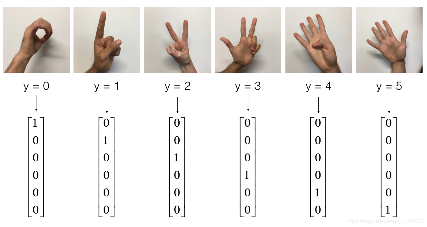
- 查看图片
# Example of a picture
index = 7
plt.imshow(X_train_orig[index])
print ("y = " + str(np.squeeze(Y_train_orig[:, index])))
y = 1

- 了解数据维度
X_train = X_train_orig/255. # 归一化
X_test = X_test_orig/255.
Y_train = convert_to_one_hot(Y_train_orig, 6).T
Y_test = convert_to_one_hot(Y_test_orig, 6).T
print ("number of training examples = " + str(X_train.shape[0]))
print ("number of test examples = " + str(X_test.shape[0]))
print ("X_train shape: " + str(X_train.shape))
print ("Y_train shape: " + str(Y_train.shape))
print ("X_test shape: " + str(X_test.shape))
print ("Y_test shape: " + str(Y_test.shape))
conv_layers = {

    }
输出:
number of training examples = 1080
number of test examples = 120
X_train shape: (1080, 64, 64, 3)
Y_train shape: (1080, 6)
X_test shape: (120, 64, 64, 3)
Y_test shape: (120, 6)
1.1 创建 placeholder
placeholder给输入数据创建一个位子,后面给他 feed 数据,样本数量维度可以置为None
# GRADED FUNCTION: create_placeholders

def create_placeholders(n_H0, n_W0, n_C0, n_y):
    """
    Creates the placeholders for the tensorflow session.

    Arguments:
    n_H0 -- scalar, height of an input image
    n_W0 -- scalar, width of an input image
    n_C0 -- scalar, number of channels of the input
    n_y -- scalar, number of classes

    Returns:
    X -- placeholder for the data input, of shape [None, n_H0, n_W0, n_C0] and dtype "float"
    Y -- placeholder for the input labels, of shape [None, n_y] and dtype "float"
    """

    ### START CODE HERE ### (≈2 lines)
    X = tf.placeholder(tf.float32, shape=(None, n_H0, n_W0, n_C0), name='X')
    Y = tf.placeholder(tf.float32, shape=(None, n_y), name='Y')
    ### END CODE HERE ###

    return X, Y
1.2 初始化参数
初始化权重/过滤器 W 1 , W 2 W_1, W_2 W1,W2 tf.contrib.layers.xavier_initializer(seed = 0)
TensorFlow 会处理偏置,你无需担心,还会自动初始化全连接层
W = tf.get_variable("W", [1,2,3,4], initializer = ...)
# GRADED FUNCTION: initialize_parameters

def initialize_parameters():
    """
    Initializes weight parameters to build a neural network with tensorflow. The shapes are:
                        W1 : [4, 4, 3, 8]
                        W2 : [2, 2, 8, 16]
    Returns:
    parameters -- a dictionary of tensors containing W1, W2
    """

    tf.set_random_seed(1)                              # so that your "random" numbers match ours

    ### START CODE HERE ### (approx. 2 lines of code)
    W1 = tf.get_variable(name='W1', shape=[4,4,3,8], dtype=tf.float32, initializer=tf.contrib.layers.xavier_initializer(seed=0))
    W2 = tf.get_variable(name='W2', shape=[2,2,8,16], dtype=tf.float32, initializer=tf.contrib.layers.xavier_initializer(seed=0))
    ### END CODE HERE ###

    parameters = {

    "W1": W1,
                  "W2": W2}

    return parameters
tf.reset_default_graph()
with tf.Session() as sess_test:
    parameters = initialize_parameters()
    init = tf.global_variables_initializer()
    sess_test.run(init)
    print("W1 = " + str(parameters["W1"].eval()[1,1,1]))
    print("W2 = " + str(parameters["W2"].eval()[1,1,1]))
输出:
W1 = [ 0.00131723  0.1417614  -0.04434952  0.09197326  0.14984085 -0.03514394
 -0.06847463  0.05245192]
W2 = [-0.08566415  0.17750949  0.11974221  0.16773748 -0.0830943  -0.08058
 -0.00577033 -0.14643836  0.24162132 -0.05857408 -0.19055021  0.1345228
 -0.22779644 -0.1601823  -0.16117483 -0.10286498]
1.3 前向传播
tf.nn.conv2d(X,W1, strides = [1,s,s,1], padding = 'SAME'),strides是各维度的步长,参考TF文档tf.nn.max_pool(A, ksize = [1,f,f,1], strides = [1,s,s,1], padding = 'SAME'),ksize是窗口大小fxf,参考TF文档tf.nn.relu(Z1),激活函数tf.contrib.layers.flatten(P),将输入 P,展平成一维向量 shape = [batch_size, k],参考TF文档tf.contrib.layers.fully_connected(F, num_outputs),给一个展平的 F 输入,返回用全连接层计算后的输出,参考TF文档(注:当训练模型时,该模块会自动初始化权重,并训练,你无需初始化它)
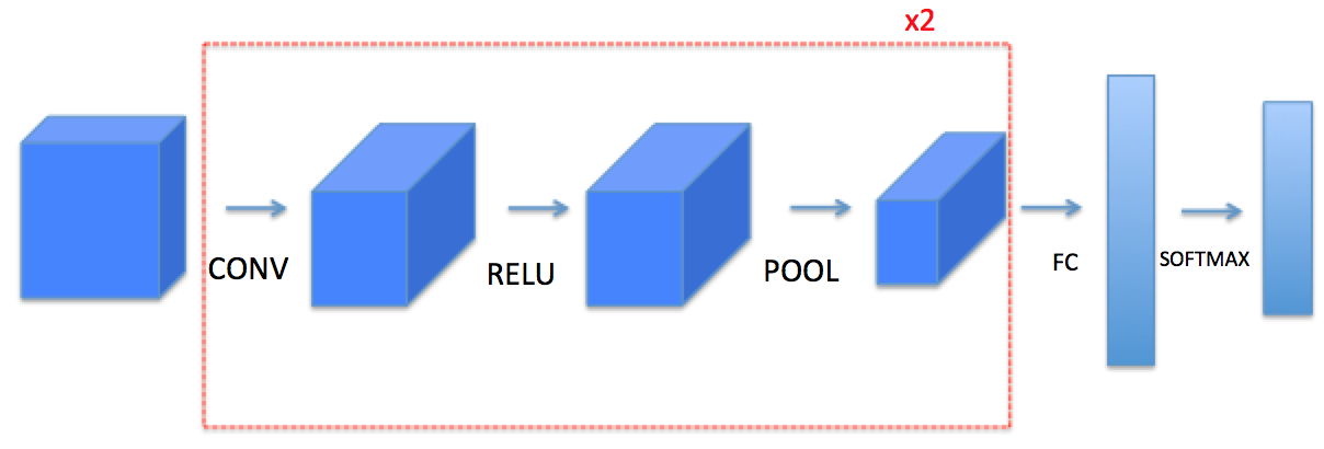
模型架构:CONV2D -> RELU -> MAXPOOL -> CONV2D -> RELU -> MAXPOOL -> FLATTEN -> FULLYCONNECTED
参数如下:
- Conv2D: stride 1, padding is “SAME”
- ReLU
- Max pool: Use an 8 by 8 filter size and an 8 by 8 stride, padding is “SAME”
- Conv2D: stride 1, padding is “SAME”
- ReLU
- Max pool: Use a 4 by 4 filter size and a 4 by 4 stride, padding is “SAME”
- Flatten the previous output.
- FULLYCONNECTED (FC) layer: Apply a fully connected layer without an non-linear activation function. (不要计算激活输出,TF有模块会一起计算 激活和cost)
# GRADED FUNCTION: forward_propagation

def forward_propagation(X, parameters):
    """
    Implements the forward propagation for the model:
    CONV2D -> RELU -> MAXPOOL -> CONV2D -> RELU -> MAXPOOL -> FLATTEN -> FULLYCONNECTED

    Arguments:
    X -- input dataset placeholder, of shape (input size, number of examples)
    parameters -- python dictionary containing your parameters "W1", "W2"
                  the shapes are given in initialize_parameters

    Returns:
    Z3 -- the output of the last LINEAR unit
    """

    # Retrieve the parameters from the dictionary "parameters"
    W1 = parameters['W1']
    W2 = parameters['W2']

    ### START CODE HERE ###
    # CONV2D: stride of 1, padding 'SAME'
    Z1 = tf.nn.conv2d(X, W1, strides=[1,1,1,1], padding='SAME')
    # RELU
    A1 = tf.nn.relu(Z1)
    # MAXPOOL: window 8x8, sride 8, padding 'SAME'
    P1 = tf.nn.max_pool(A1, ksize=[1,8,8,1],strides=[1,8,8,1],padding='SAME')
    # CONV2D: filters W2, stride 1, padding 'SAME'
    Z2 = tf.nn.conv2d(P1, W2, strides=[1,1,1,1],padding='SAME')
    # RELU
    A2 = tf.nn.relu(Z2)
    # MAXPOOL: window 4x4, stride 4, padding 'SAME'
    P2 = tf.nn.max_pool(A2, ksize=[1,4,4,1],strides=[1,4,4,1],padding='SAME')
    # FLATTEN
    P2 = tf.contrib.layers.flatten(P2)
    # FULLY-CONNECTED without non-linear activation function (not not call softmax).
    # 6 neurons in output layer. Hint: one of the arguments should be "activation_fn=None"
    Z3 = tf.contrib.layers.fully_connected(P2, num_outputs=6, activation_fn=None)
    ### END CODE HERE ###

    return Z3
tf.reset_default_graph()

with tf.Session() as sess:
    np.random.seed(1)
    X, Y = create_placeholders(64, 64, 3, 6)
    parameters = initialize_parameters()
    Z3 = forward_propagation(X, parameters)
    init = tf.global_variables_initializer()
    sess.run(init)
    a = sess.run(Z3, {

    X: np.random.randn(2,64,64,3), Y: np.random.randn(2,6)})
    print("Z3 = " + str(a))
输出:(可能是版本原因,跟标准答案不一样)
Z3 = [[ 1.4416984  -0.24909666  5.450499   -0.2618962  -0.20669907  1.3654671 ]
 [ 1.4070846  -0.02573211  5.08928    -0.48669922 -0.40940708  1.2624859 ]]
1.4 计算损失
tf.nn.softmax_cross_entropy_with_logits(logits = Z3, labels = Y),计算softmax激活 及 熵损失tf.reduce_mean,计算均值
# GRADED FUNCTION: compute_cost

def compute_cost(Z3, Y):
    """
    Computes the cost

    Arguments:
    Z3 -- output of forward propagation (output of the last LINEAR unit), of shape (6, number of examples)
    Y -- "true" labels vector placeholder, same shape as Z3

    Returns:
    cost - Tensor of the cost function
    """

    ### START CODE HERE ### (1 line of code)
    cost = tf.reduce_mean(tf.nn.softmax_cross_entropy_with_logits(logits=Z3, labels=Y))
    ### END CODE HERE ###

    return cost
tf.reset_default_graph()

with tf.Session() as sess:
    np.random.seed(1)
    X, Y = create_placeholders(64, 64, 3, 6)
    parameters = initialize_parameters()
    Z3 = forward_propagation(X, parameters)
    cost = compute_cost(Z3, Y)
    init = tf.global_variables_initializer()
    sess.run(init)
    a = sess.run(cost, {

    X: np.random.randn(4,64,64,3), Y: np.random.randn(4,6)})
    print("cost = " + str(a))
输出:
cost = 4.6648693 # 跟标准答案不一样
1.5 模型
- 创建 placeholders
- 初始化参数
- 前向传播
- 计算损失
- 创建优化器
# GRADED FUNCTION: model

def model(X_train, Y_train, X_test, Y_test, learning_rate = 0.009,
          num_epochs = 100, minibatch_size = 64, print_cost = True):
    """
    Implements a three-layer ConvNet in Tensorflow:
    CONV2D -> RELU -> MAXPOOL -> CONV2D -> RELU -> MAXPOOL -> FLATTEN -> FULLYCONNECTED

    Arguments:
    X_train -- training set, of shape (None, 64, 64, 3)
    Y_train -- test set, of shape (None, n_y = 6)
    X_test -- training set, of shape (None, 64, 64, 3)
    Y_test -- test set, of shape (None, n_y = 6)
    learning_rate -- learning rate of the optimization
    num_epochs -- number of epochs of the optimization loop
    minibatch_size -- size of a minibatch
    print_cost -- True to print the cost every 100 epochs

    Returns:
    train_accuracy -- real number, accuracy on the train set (X_train)
    test_accuracy -- real number, testing accuracy on the test set (X_test)
    parameters -- parameters learnt by the model. They can then be used to predict.
    """

    ops.reset_default_graph()      # to be able to rerun the model without overwriting tf variables
    tf.set_random_seed(1)          # to keep results consistent (tensorflow seed)
    seed = 3                       # to keep results consistent (numpy seed)
    (m, n_H0, n_W0, n_C0) = X_train.shape
    n_y = Y_train.shape[1]
    costs = []                     # To keep track of the cost

    # Create Placeholders of the correct shape
    ### START CODE HERE ### (1 line)
    X, Y = create_placeholders(n_H0, n_W0, n_C0, n_y)
    ### END CODE HERE ###

    # Initialize parameters
    ### START CODE HERE ### (1 line)
    parameters = initialize_parameters()
    ### END CODE HERE ###

    # Forward propagation: Build the forward propagation in the tensorflow graph
    ### START CODE HERE ### (1 line)
    Z3 = forward_propagation(X, parameters)
    ### END CODE HERE ###

    # Cost function: Add cost function to tensorflow graph
    ### START CODE HERE ### (1 line)
    cost = compute_cost(Z3, Y)
    ### END CODE HERE ###

    # Backpropagation: Define the tensorflow optimizer. Use an AdamOptimizer that minimizes the cost.
    ### START CODE HERE ### (1 line)
    optimizer = tf.train.AdamOptimizer(learning_rate=learning_rate).minimize(cost)
    ### END CODE HERE ###

    # Initialize all the variables globally
    init = tf.global_variables_initializer()

    # Start the session to compute the tensorflow graph
    with tf.Session() as sess:

        # Run the initialization
        sess.run(init)

        # Do the training loop
        for epoch in range(num_epochs):

            minibatch_cost = 0.
            num_minibatches = m // minibatch_size
            # number of minibatches of size minibatch_size in the train set
            seed = seed + 1
            minibatches = random_mini_batches(X_train, Y_train, minibatch_size, seed)

            for minibatch in minibatches:

                # Select a minibatch
                (minibatch_X, minibatch_Y) = minibatch
                # IMPORTANT: The line that runs the graph on a minibatch.
                # Run the session to execute the optimizer and the cost, the feedict should contain a minibatch for (X,Y).
                ### START CODE HERE ### (1 line)
                _ , temp_cost = sess.run([optimizer, cost], feed_dict={

    X:minibatch_X, Y:minibatch_Y})
                ### END CODE HERE ###

                minibatch_cost += temp_cost / num_minibatches


            # Print the cost every epoch
            if print_cost == True and epoch % 5 == 0:
                print ("Cost after epoch %i: %f" % (epoch, minibatch_cost))
            if print_cost == True and epoch % 1 == 0:
                costs.append(minibatch_cost)


        # plot the cost
        plt.plot(np.squeeze(costs))
        plt.ylabel('cost')
        plt.xlabel('iterations (per tens)')
        plt.title("Learning rate =" + str(learning_rate))
        plt.show()

        # Calculate the correct predictions
        predict_op = tf.argmax(Z3, 1)
        correct_prediction = tf.equal(predict_op, tf.argmax(Y, 1))

        # Calculate accuracy on the test set
        accuracy = tf.reduce_mean(tf.cast(correct_prediction, "float"))
        print(accuracy)
        train_accuracy = accuracy.eval({

    X: X_train, Y: Y_train})
        test_accuracy = accuracy.eval({

    X: X_test, Y: Y_test})
        print("Train Accuracy:", train_accuracy)
        print("Test Accuracy:", test_accuracy)

        return train_accuracy, test_accuracy, parameters
- 训练模型 100 epochs
_, _, parameters = model(X_train, Y_train, X_test, Y_test)
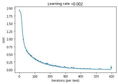
使用作业默认的学习率(0.009)和迭代次数(100),效果很差,只有60%,50%多的训练准确率和测试准确率
更改为:learning_rate = 0.002, num_epochs = 600
Cost after epoch 0: 1.943088
Cost after epoch 5: 1.885871
Cost after epoch 10: 1.824765
Cost after epoch 15: 1.595936
Cost after epoch 20: 1.243416
Cost after epoch 25: 1.004351
Cost after epoch 30: 0.875302
Cost after epoch 35: 0.767196
Cost after epoch 40: 0.711865
Cost after epoch 45: 0.640964
Cost after epoch 50: 0.574520
。。。。
Cost after epoch 150: 0.207593
。。。。
Cost after epoch 300: 0.071819
。。。。
Cost after epoch 500: 0.013352
。。。。
Cost after epoch 595: 0.016594
Tensor("Mean_1:0", shape=(), dtype=float32)
Train Accuracy: 0.9916667
Test Accuracy: 0.9
训练集上准确率为 99%,测试集上准确率为 90%,存在一定的过拟合。
fname = "images/thumbs_up.jpg"
image = np.array(ndimage.imread(fname, flatten=False))
my_image = scipy.misc.imresize(image, size=(64,64))
plt.imshow(my_image)

一起加油学习!冲啊!
我的CSDN博客地址 https://michael.blog.csdn.net/
长按或扫码关注我的公众号(Michael阿明),一起加油、一起学习进步!