文章目录

卷积神经网络作业

卷积神经网络作业

1. 高斯拉普拉斯算子(边缘检测)

作业要求

输入一张图片，使用高斯拉普拉斯算子代替卷积，进行卷积操作，输出处理后的图片

输入：一张图片

输出：经过高斯拉普拉斯算子处理后的图片

1.1 简介

拉普拉斯算子（Laplace Operator）是n维欧几里德空间中的一个二阶微分算子，定义为梯度 $\nabla f$ 的散度 $(\nabla \cdot f)$ 。如果 $f$ 是二阶可微的实函数，则 $f$ 的拉普拉斯算子定义为
$\Delta f=\nabla^2f=\nabla\cdot\nabla f$

1.2 拉普拉斯算子

Laplace算子作为一种优秀的边缘检测算子，是具有旋转不变性的各向同性算子，拉普拉斯算子广泛用于图像增强，图像锐化中。该方法通过对图像求图像的二阶倒数的零交叉点来实现边缘的检测，

记图片像素的强度值为 $I (x, y)$ ,其所对应的拉普拉斯算子 $L (x, y)$ 如下所示：
$L(x,y)=\frac{\partial^2 I}{\partial x^2}+\frac{\partial^2I}{\partial y^2}$
由于图片是采用离散的像素值进行表示的，因此我们可以寻找一个近似于拉普拉斯算子的二阶导数离散卷积核。此时采用差分近似来使用拉普拉斯算子，

一维二阶差分
$f^\prime(x)=(f(x+1)-f(x))-(f(x)-f(x-1))=f(x-1)-2f(x)+f(x+1)$
二维二阶差分为：
$\nabla^2f(x,y)=f(x+1,y)+f(x-1,y)+f(x,y-1)+f(x,y-1)-4f(x,y)$
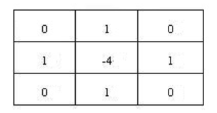
在上述近似下，这个过程可以采用卷积核进行计算。在计算时则有拉普拉斯算子4邻域，8邻域的算子模板来使用：

4邻域（较常用）

在这里插入图片描述

8邻域

在这里插入图片描述

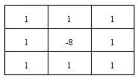
由模板知，当邻域像素灰度值相同时，filter的卷积结果为0；

当中心像素的灰度较其他灰度值高或当中心像素的灰度较其他灰度值低时，filter的卷积运算结果非0。

如果在图像中一个较暗的区域中出现了一个亮点，拉普拉斯算子会产生"亮者更亮"的效果，故这也是拉普拉斯算子在图像锐化的原理。

1.3 高斯拉普拉斯算子

由于Laplace算子是通过对图像进行微分操作实现边缘检测的，所以对离散点和噪声比较敏感。

于是，首先对图像进行高斯卷积滤波进行降噪处理，再采用Laplace算子进行边缘检测，就可以提高算子对噪声和离散点的鲁棒性，如此，拉普拉斯高斯算子Log（Laplace of Gaussian）就诞生了。
$G_{\sigma}(x,y)=\frac{1}{2\pi \sigma^2}exp(-\frac{x^2+y^2}{2\sigma^2})$
先利用高斯平滑滤波进行处理，可以降低图片中的高频噪声，方便后续的拉普拉斯操作。

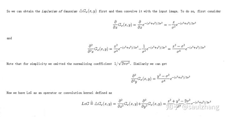
事实上由于卷积操作具有结合律，因此我们先将高斯平滑滤波器与拉普拉斯滤波器进行卷积，然后利用得到的混合滤波器去对图片进行卷积以得到所需的结果。采用这个做法主要有以下两个优点：

由于高斯和拉普拉斯核通常都比图像小得多，所以这种方法通常只需要很少的算术运算。
LoG (’ Laplacian of Gaussian’)内核的参数可以预先计算，因此在运行时只需要对图像执行一遍的卷积即可。

以0为中心，高斯标准差为 $\sigma$ 的二维的 $L o G$ 函数的表达式如下所示
$LoG(x,y)=-\frac{1}{\pi\sigma ^4}[1-\frac{x^2+y^2}{2\sigma^2}]e^{-\frac{x^2+y^2}{2\sigma^2}}$
具体的推导过程如下所示:

函数的图像如下图所示：

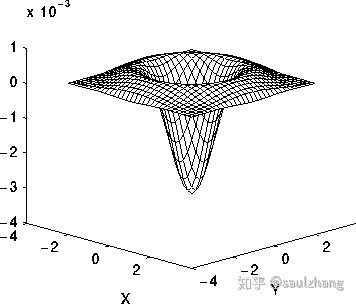
以下图3所示的离散卷积核可以近似上面的表达式(当 $\sigma=1.4$ 时)：

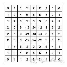
值得注意的是，随着高斯函数变得越来越窄，LoG卷积核将会近似于图1中所示的简单Laplacian内核，主要原因是因为采用十分窄的高斯函数( $\sigma<0.5 pixels$ 时，其在于离散的网格上面是不起作用的。因此，在离散的网格上，简单的拉普拉斯算子可以看成是一种高斯函数很窄的 $L o G$ 函数。

1.3 LoG使用指南

$L o G$ 运算计算图片在空间上的二阶导数。这意味着图片中某个区域的强度是固定值的时候，其 $L o G$ 变换的响应值为0。而在图片的强度发生变化的区域，在较暗的一侧 $L o G$ 的响应值是正数，而在较亮的一侧, $L o G$ 的响应值则为负数，这意味着在两个强度均匀但不同的区域中间会有一条相对锐利的边，而 $L o G$ 函数对于这一部分区域的响应为：

在连续强度不变的区域响应值为0
在边的一侧响应为正
在边的另一侧响应为负
在边中间的某一点响应值为0

以下的图4展示了 $L o G$ 对于图像中边缘的响应

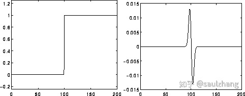
因此可以看出 $L o G$ 过滤器本身的作用就是突出图像中的边缘。

例如下图5的 $L o G$ 变换的响应为图6

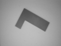
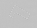
其中 $L o G$ 卷积核的高斯标准差 $\sigma=1$ ,卷积核的大小为 $7\times 7$ 需要注意的是，由于 $L o G$ 卷积核的输出包含负数值，因此需要将最后输出的结果归一化到0~255之间。如果将经过过滤的部分图像或梯度图像添加到原始图像中，那么结果将使原始图像中的任何边缘更清晰和具有更高的对比度，这常常在遥感应用中作为图像增强的技巧。以图7为例：

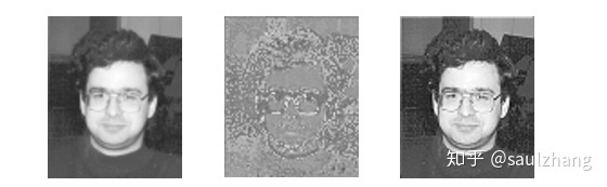
图7.左边为原始图片，中间为LoG变换输出的图片，右边为左边的图片和中间的图片相结合结果

值得一提的是增强之后图像的边缘变得更加的锋利但也带来了一定的噪声，以下图8展示了噪声对 $L o G$ 变换的影响。

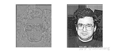
图8. 左图为LoG对原始图片的变换结果，右图为LoG对增强后的图片的变换结果

从图8中可以使用右图这种锐化的图像进行边缘增强，得到的是有噪声的结果。相反，扩大算子的高斯平滑分量可以减少部分噪声，但同时会使得增强效果不那么明显。注意，由于 $L o G$ 是一个各向同性的过滤器，所以不可能直接从 $L o G$ 输出中提取边缘的方向信息，这与其他边缘检测器(如Roberts Cross和Sobel算子)的方法类似。

1.4 总结

拉普拉斯算子是图像二阶空间导数的二维各向同性测度。
拉普拉斯算子可以突出图像中强度发生快速变化的区域，因此常用在边缘检测任务当中。在进行Laplacian操作之前通常需要先用高斯平滑滤波器对图像进行平滑处理，以降低Laplacian操作对于噪声的敏感性。
该操作通常是输入一张灰度图，经过处理之后输出一张灰度图。

1.5 代码实现

采用所示的近似矩阵来作为 $L o G$ 变换的近似卷积核：

import torch
import torch.nn.functional as F
import numpy as np

from torch.autograd import Variable
from math import exp
from PIL import Image
from torchvision.utils import save_image, make_grid

#将最后的矩阵中的元素归一化到0~1之间
def minmaxscaler(data):
    min = torch.min(data)
    max = torch.max(data)    
    return (data - min)/(max-min)

#LoG变换
def LoG(img,window,window_size,mode="RGB"):
    img1_array = np.array(img,dtype=np.float32)#Image -> array
    img1_tensor = torch.from_numpy(img1_array)# array -> tensor
    # 处理不同通道数的数据
    if mode == 'L':
        img1_tensor = img1_tensor.unsqueeze(0).unsqueeze(0)#h,w -> n,c,h,w 
    else:#RGB or RGBA
        img1_tensor = img1_tensor.permute(2,0,1)# h,w,c -> c,h,w 
        img1_tensor = img1_tensor.unsqueeze(0)#c,h,w -> n,c,h,w 
    channel = img1_tensor.size()[1]
    window = Variable(window.expand(channel, 1, window_size, window_size).contiguous())
    output = F.conv2d(img1_tensor, window, padding = window_size//2, groups = channel)
    output = minmaxscaler(output)# 归一化到0~1之间
    if (channel==4):
        save_image(output, "output.png", normalize=False)
    else:
        save_image(output, "output.jpg", normalize=False)
    return output

#近似卷积核
window  = torch.Tensor([[[0,1,1,2,2,2,1,1,0],
                        [1,2,4,5,5,5,4,2,1],
                        [1,4,5,3,0,3,5,4,1],
                        [2,5,3,-12,-24,-12,3,5,2],
                        [2,5,0,-24,-40,-24,0,5,2],
                        [2,5,3,-12,-24,-12,3,5,2],
                        [1,4,5,3,0,3,4,4,1],
                        [1,2,4,5,5,5,4,2,1],
                        [0,1,1,2,2,2,1,1,0]]])
window_size = 9
img = Image.open("./input.png")
img = img.convert('L') 
LoG(img,window,window_size,img.mode)

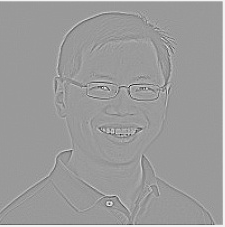
结果

2. 使用LeNet网络，输出特征图

2.1 作业要求

使用预训练好的模型，输入图片，对模型某一层的特征图进行输出

输入：一张图片

输出：某一层的特征图图片

首先贴一下vgg的网络架构

2.2 代码实现

首先vgg网络

import torch.nn as nn
import torch


class SE_VGG(nn.Module):
    def __init__(self, num_classes):
        super().__init__()
        self.num_classes = num_classes
        # define an empty for Conv_ReLU_MaxPool
        net = []

        # block 1
        net.append(nn.Conv2d(in_channels=3, out_channels=64, padding=1, kernel_size=3, stride=1))
        net.append(nn.ReLU())
        net.append(nn.Conv2d(in_channels=64, out_channels=64, padding=1, kernel_size=3, stride=1))
        net.append(nn.ReLU())
        net.append(nn.MaxPool2d(kernel_size=2, stride=2))

        # block 2
        net.append(nn.Conv2d(in_channels=64, out_channels=128, kernel_size=3, stride=1, padding=1))
        net.append(nn.ReLU())
        net.append(nn.Conv2d(in_channels=128, out_channels=128, kernel_size=3, stride=1, padding=1))
        net.append(nn.ReLU())
        net.append(nn.MaxPool2d(kernel_size=2, stride=2))

        # block 3
        net.append(nn.Conv2d(in_channels=128, out_channels=256, kernel_size=3, padding=1, stride=1))
        net.append(nn.ReLU())
        net.append(nn.Conv2d(in_channels=256, out_channels=256, kernel_size=3, padding=1, stride=1))
        net.append(nn.ReLU())
        net.append(nn.Conv2d(in_channels=256, out_channels=256, kernel_size=3, padding=1, stride=1))
        net.append(nn.ReLU())
        net.append(nn.MaxPool2d(kernel_size=2, stride=2))

        # block 4
        net.append(nn.Conv2d(in_channels=256, out_channels=512, kernel_size=3, padding=1, stride=1))
        net.append(nn.ReLU())
        net.append(nn.Conv2d(in_channels=512, out_channels=512, kernel_size=3, padding=1, stride=1))
        net.append(nn.ReLU())
        net.append(nn.Conv2d(in_channels=512, out_channels=512, kernel_size=3, padding=1, stride=1))
        net.append(nn.ReLU())
        net.append(nn.MaxPool2d(kernel_size=2, stride=2))

        # block 5
        net.append(nn.Conv2d(in_channels=512, out_channels=512, kernel_size=3, padding=1, stride=1))
        net.append(nn.ReLU())
        net.append(nn.Conv2d(in_channels=512, out_channels=512, kernel_size=3, padding=1, stride=1))
        net.append(nn.ReLU())
        net.append(nn.Conv2d(in_channels=512, out_channels=512, kernel_size=3, padding=1, stride=1))
        net.append(nn.ReLU())
        net.append(nn.MaxPool2d(kernel_size=2, stride=2))

        # add net into class property
        self.extract_feature = nn.Sequential(*net)

        # define an empty container for Liqnear operations
        classifier = []
        classifier.append(nn.Linear(in_features=512*7*7, out_features=4096))
        classifier.append(nn.ReLU())
        classifier.append(nn.Dropout(p=0.5))
        classifier.append(nn.Linear(in_features=4096, out_features=4096))
        classifier.append(nn.ReLU())
        classifier.append(nn.Dropout(p=0.5))
        classifier.append(nn.Linear(in_features=4096, out_features=self.num_classes))

        # add classifier into class property
        self.classifier = nn.Sequential(*classifier)


    def forward(self, x):
        feature = self.extract_feature(x)
        feature = feature.view(x.size(0), -1)
        classify_result = self.classifier(feature)
        return classify_result

if __name__ == "__main__":
    x = torch.rand(size=(8, 3, 224, 224))
    vgg = SE_VGG(num_classes=1000)
    out = vgg(x)
    print(out.size())

但是呢？由于需要输出特征图，所以我们得使用别人预训练好的模型

import cv2
import numpy as np
import torchvision
from torch.utils.data import DataLoader
from torchvision.models import vgg16_bn
import torch
import torch.nn as nn
import os
from torchvision.transforms import transforms
from PIL import Image


# 加载数据集
def get_dataloader(mode):
    """
    获取数据集加载
    :param mode:
    :return:
    """
    # 准备数据迭代器
    # 这里我已经下载好了，所以是否需要下载写的是false
    # 准备数据集，其中0.1307，0.3081为MNIST数据的均值和标准差，这样操作能够对其进行标准化
    # 因为MNIST只有一个通道（黑白图片）,所以元组中只有一个值
    dataset = torchvision.datasets.MNIST('./mini',
                                         train=mode,
                                         download=False,
                                         transform=torchvision.transforms.Compose([
                                             torchvision.transforms.ToTensor(),
                                             torchvision.transforms.Normalize(
                                                 (0.1307,), (0.3081,))
                                         ]))

    return DataLoader(dataset, batch_size=64, shuffle=True)


# 图像预处理函数，将图像转换成[224,224]大小,并进行Normalize,返回[1,3.224,224]的四维张量
def preprocess_image(cv2im, resize_im=True):
    # 在ImageNet100万张图像上计算得到的图像的均值和标准差，它会使图像像素值大小在[2.7.2.1]之间，但是整体图像像素值的分布会是标准正态分布(（均值为0，方差为1)
    # 之所以使用这种方法，是因为这是基于 lmageNet的预训练VGG16对输入图像的要求
    mean = [0.485, 0.456, 0.406]
    std = [0.229, 0.224, 0.225]

    # 改变图像大小并进行Normalize
    if resize_im:
        cv2im = cv2.resize(cv2im, dsize=(224, 224), interpolation=cv2.INTER_CUBIC)
    im_as_arr = np.float32(cv2im)
    im_as_arr = np.ascontiguousarray(im_as_arr[..., ::-1])
    im_as_arr = im_as_arr.transpose(2, 0, 1)  # 将[W,H,CJ的次序改变为[C,W,H]

    for channel, _ in enumerate(im_as_arr):  # 进行在ImageNet上预训练的VGG16要求的ImageNe输入图像的Normalizeim_as_arr[channel] /= 255
        im_as_arr[channel] /= 255
        im_as_arr[channel] -= mean[channel]
        im_as_arr[channel] /= std[channel]

    # 转变为三维 Tensor,[C,W, H
    im_as_ten = torch.from_numpy(im_as_arr).float()
    im_as_ten = im_as_ten.unsqueeze_(0)  # 扩充为四维Tensor,变为[1,C,W,H

    return im_as_ten  # 返回处理好的[1,3,224,224]四维Tensor


class FeaureVisualization():
    def __init__(self, img_path, selected_layer):
        """

        :param img_path: 图片的地址
        :param selected_layer: 期望输出的特征图
        """
        self.img_path = img_path
        self.select_layer = selected_layer
        # 如果预训练模型已经下载好了，就加载本地
        if os.path.exists("./model/vgg16.pth"):
            self.model = vgg16_bn(pretrained=False)
            self.model.load_state_dict(torch.load(r"./model/vgg16.pth"))
            self.model = self.model.features
        else:
            self.model = vgg16_bn(pretrained=True).features

    def preprocess_image2(self):
        """
        加载图片，把图片进行归一化处理，变成[0,1]之间
        返回[1,C,H,W]格式的tensor形式
        :return:
        """
        mean = [0.485, 0.456, 0.406]
        std = [0.229, 0.224, 0.225]
        T = transforms.Compose([
            transforms.Resize(size=(224, 224)),
            transforms.ToTensor(),
            transforms.Normalize(mean=mean, std=std)
        ])
        return T(Image.open(self.img_path)).unsqueeze(0)

    def get_features(self):
        """
        获取特征图信息
        :return:
        """
        x = self.preprocess_image2()  # 获取图片信息
        print(x.shape)
        for index, layer in enumerate(self.model):
            x = layer(x)
            if index == self.select_layer:
                return x

    def get_single_feature(self):
        return self.get_features()

    def save_feature_to_img(self):
        features = self.get_features()
        print(features.shape)
        for i in range(features.shape[1]):

            feature = features[:, i, :, :].squeeze().data.numpy()
            # batch为1,所以所以直接view成二维的
            # #根据图像的像素值中最大最小值，将特征图的像素值归一化到了[0,1];
            feature = (feature - np.amin(feature)) / (np.amax(feature) - np.amin(feature + 1e-5))
            feature = np.round(feature * 255)

            if not os.path.exists("./image"):
                os.path.exists("./image")

            cv2.imwrite("./image/{}.jpg".format(i), feature)


if __name__ == '__main__':
    myClass = FeaureVisualization("./input.jpg", 0)
    print(myClass.model)

    myClass.save_feature_to_img()

这里我们输出第一层的特征图信息.

这就是其中的一幅图片信息

参考资料

高斯拉普拉斯算子（Laplacian of Gaussian, LoG） - 知乎 (zhihu.com)

机器学习–拉普拉斯算子（Laplace Operator）学习整理_Mr.琛的博客-CSDN博客_拉普拉斯算子例题