python--逻辑回归实例操作

以下内容笔记出自‘跟着迪哥学python数据分析与机器学习实战’，外加个人整理添加，仅供个人复习使用。

---

基于信用卡交易记录数据建立分类模型预测哪些交易是正常的，哪些交易是异常的。

流程：

• 加载数据，观察问题；
• 针对问题给出解决方案；
• 数据集切分；
• 逻辑回归模型；

---

导入数据

import pandas as pd
import matplotlib.pyplot as plt
import numpy as np
%matplotlib inline

file=r'creditcard.csv'
data=pd.read_csv(file)
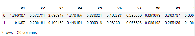
print(data.shape)
data.head(6)

目标是分类模型，首先查看标签分布：

#查看标签分布
count_classes=pd.value_counts(data['Class'],sort=True).sort_index()
#pd.value_counts()函数要比转换为dataframe在sort.values()简洁
count_classes.plot(kind='bar')  #pandas自带作图函数
plt.xlabel('Class')
plt.ylabel('Frequency')

数据标准化

观察数据特征，列Amount值数量级较大，其余列均0-1，对其进行标准化。

from sklearn.preprocessing import StandardScaler
data['normAmount']=StandardScaler().fit_transform(data['Amount'].values.reshape(-1,1))
data=data.drop(['Time','Amount'],axis=1)
data.head(2)

数据下采样方案

data['Class'].value_counts()

0 284315
1 492
Name: Class, dtype: int64
由于数据标签很不平衡，建立的模型有偏，进行下采样。

X=data.iloc[:,data.columns!='Class']
y=data.iloc[:,data.columns=='Class']

#得到所有标签为1（异常）样本的索引
num_fraud=len(data[data.Class==1])
fraud_index=np.array(data[data.Class==1].index)

#得到标签为0（正常）样本的索引
normal_index=data[data.Class==0].index

#在正常样本中随机采样出指定个数的样本，并取其索引
random_nor_index=np.random.choice(normal_index,num_fraud,replace=True)
random_nor_index=np.array(random_nor_index)

#合并所有正常和异常样本的索引，并提取数据
under_sample_index=np.concatenate([fraud_index,random_nor_index])
under_sample_data=data.iloc[under_sample_index,:]

X_undersample=under_sample_data.iloc[:,under_sample_data.columns!='Class']
y_undersample=under_sample_data.iloc[:,under_sample_data.columns=='Class']

#下采样样本比例
print('正常样本比例：',len(under_sample_data[under_sample_data.Class==0])/len(under_sample_data))
print('异常样本比例：',len(under_sample_data[under_sample_data.Class==1])/len(under_sample_data))
print('下采样总样本量:',len(under_sample_data))

正常样本比例： 0.5
异常样本比例： 0.5
下采样总样本量: 984

建立模型

#Recall=TP(TP+FN)
from sklearn.model_selection import train_test_split
from sklearn.linear_model import LogisticRegression
from sklearn.model_selection import KFold,cross_val_score  #交叉验证
from sklearn.metrics import confusion_matrix,recall_score,classification_report
from sklearn.model_selection import cross_val_predict

分割数据集

由于模型测试时使用的测试集是原始数据切分出来的测试集，而不是下采样数据切分的数据集，因此要对原始数据和下采样数据都进行切分

X_train,X_test,y_train,y_test=train_test_split(X,y,test_size=0.3,random_state=0)
print('原始训练集：',X_train.shape)
print('原始测试集：',X_test.shape)
print('原始样本：',data.shape)

X_train_under,X_test_under,y_train_under,y_test_under=\
        train_test_split(X_undersample,y_undersample,
                        test_size=0.3,random_state=0)
print('下采样训练集：',X_train_under.shape)
print('下采样测试集：',X_test_under.shape)
print('下采样样本:',under_sample_data.shape)

原始训练集： (199364, 29)
原始测试集： (85443, 29)
原始样本： (284807, 30)
下采样训练集： (688, 29)
下采样测试集： (296, 29)
下采样样本: (984, 30)

使用下采样数据建模

定义交叉验证函数
交叉验证是为了找到更合适参数的求稳操作，是对下采样训练集进行分割

正则化参数的选择：

• LogisticRegession默认带了正则项，可选择l1或l2，默认l2。调参时，主要目的是解决过拟合，一般选择l2即可。若l2正则化还是过拟合，或特征非常多，希望一些不重要的特征系数归零，让模型系数稀疏化时，可以l1正则。

import numpy as np
from sklearn.model_selection import KFold
'''
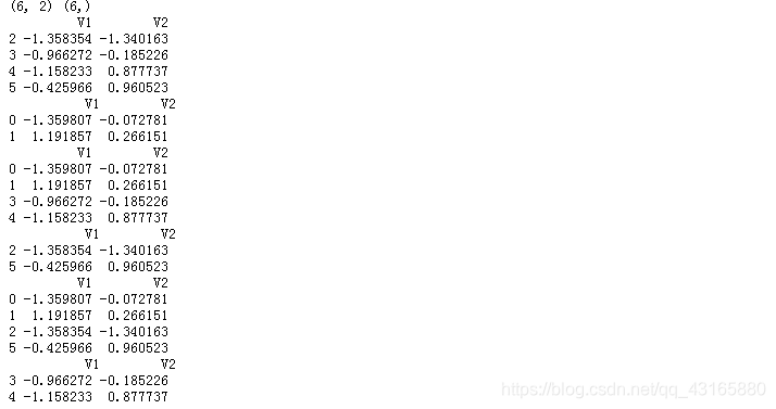
交叉验证分割数据过程
'''
a=data.loc[:,['V1','V2']][0:6]
b=data.loc[:,'Class'][0:6]
print(a.shape,b.shape)

kfold=KFold(3,shuffle=True)
index=kfold.split(X=a,y=b)

for train,test in index:
    print(a.iloc[train],'\n',a.iloc[test])

使用l2正则惩罚项，并选取不同参数进行建模

import warnings
warnings.filterwarnings('ignore')

'''利用cross_val_score函数'''
c_param_range=[0.01,0.1,1,10,100]
for c in c_param_range:
    lr=LogisticRegression(C=c,penalty='l2',random_state=0)
    scores=cross_val_score(lr,X_train_under,y_train_under,cv=5,
                           scoring='accuracy')
    #scoring参数：accuracy,roc_auc
    mean_score=np.mean(scores)
    print((c,mean_score))

(0.01, 0.9317359568390987)
(0.1, 0.9288268274621814)
(1, 0.9273669734475828)
(10, 0.921548714693748)
(100, 0.9200888606791494)

在sklearn工具包中，C参数的意义正好是倒过来的，C=0.01表示正则化力度比较大，而C=100表示力度较小。（一定要参考API文档）

下采样数据-混淆矩阵

lr=LogisticRegression(C=0.01,penalty='l2')
lr.fit(X_train_under,y_train_under)
y_pred=lr.predict(X_test_under)

#混淆矩阵
cm=confusion_matrix(y_test_under,y_pred)
cm
#混淆矩阵第一个参数是行标，第二个参数是列标

array([[148, 1],
[ 20, 127]], dtype=int64)

---

确定行列标的方式

#确定混淆矩阵的行列标
print(y_test_under.Class.value_counts())
pd.DataFrame(y_pred).iloc[:,0].value_counts()

0 149
1 147
Name: Class, dtype: int64
0 168
1 128
Name: 0, dtype: int64

---

作图：

import seaborn as sns
plt.figure(figsize=(6,4))
plt.rcParams['font.sans-serif']='SimHei'
sns.heatmap(cm,cmap='GnBu',vmin=0,vmax=150,
            annot=False,center=True,fmt='.0f')
plt.xlabel('Predicted')
plt.ylabel('True')
plt.show()

#召回率
recall=cm[1,1]/(cm[1,0]+cm[1,1])
recall

0.8639455782312925

阈值对结果的影响

#用最好的参数建模
lr=LogisticRegression(C=0.01,penalty='l2')
#下采样数据训练模型
lr.fit(X_train_under,y_train_under)
#预测值
y_pred_prob=lr.predict_proba(X_test_under)

#指定不同阈值
thresholds=[0.1,0.2,0.3,0.4,0.5,0.6,0.7,0.8,0.9]

plt.figure(figsize=(10,10))
j=1

for i in thresholds:
    y_test_pre_high_recall=y_pred_prob[:,1]>i  #得出的是True和False数据
    #plt.subplot(3,3,j)
    j+=1
    cm=confusion_matrix(y_test_under,y_test_pre_high_recall)
    print('阈值为',i,'时的召回率',cm[1,1]/(cm[1,0]+cm[1,1]))
    #sns.heatmap(cm,cmap='GnBu',annot=True)
    #plt.xlabel('Predicted')
    #plt.ylabel('True')
    print(cm)

原始数据建模结果

lr=LogisticRegression(C=0.01,penalty='l2')
lr.fit(X_train,y_train)
y_pred=lr.predict(X_test)

cm2=confusion_matrix(y_test,y_pred)
print('召回率',cm2[1,1]/(cm2[1,0]+cm2[1,1]))
sns.heatmap(cm2,cmap='GnBu')
plt.xlabel('Predicted')
plt.ylabel('True')
plt.show()

过采样策略

同样可以采用过采样策略进行建模

import pandas as pd
from imblearn.over_sampling import SMOTE
from sklearn.metrics import confusion_matrix
from sklearn.model_selection import train_test_split

features=data.iloc[:,data.columns!='Class']
labels=data['Class']
print(features.shape)
print(labels.shape)

(284807, 29)
(284807,)

features_train,features_test,labels_train,labels_test=train_test_split(features,labels,
                                                                      test_size=0.3,
                                                                      random_state=0)

利用SMOTE算法进行样本生成，正例和负例样本数量一致

oversampler=SMOTE(random_state=0)
os_features,os_labels=oversampler.fit_sample(features_train,labels_train)

print(len(os_labels[os_labels==0]))
print(len(os_labels[os_labels==1]))

199019
199019

建立模型

import warnings
warnings.filterwarnings('ignore')

'''利用cross_val_score函数'''
c_param_range=[0.01,0.1,1,10,100]
for c in c_param_range:
    lr=LogisticRegression(C=c,penalty='l2',random_state=0)
    scores=cross_val_score(lr,os_features,os_labels,cv=5,
                           scoring='accuracy')
    #scoring参数：accuracy,roc_auc
    mean_score=np.mean(scores)
    print((c,mean_score))

(0.01, 0.9442515545639256)
(0.1, 0.9450153010987146)
(1, 0.945188651552278)
(10, 0.9452162870604811)
(100, 0.94522633639644)

选择最好参数建模

lr=LogisticRegression(C=1,penalty='l2')
lr.fit(os_features,os_labels)
y_pred=lr.predict(features_test)

cm=confusion_matrix(labels_test,y_pred)
print(cm)
print('召回率',cm[1,1]/(cm[1,0]+cm[1,1]))
print('准确率',lr.score(features_test,labels_test))
sns.heatmap(cm,cmap='GnBu')