基本全局阈值处理
1、全局阈值处理
(1)计算步骤
通常,在图像处理中首选的方法是使用一种能基于图像数据自动地选择阈值的算法,为了自动选阈值,下列迭代过程采用的就是这样的方法:
(1) 针对全局阈值选择初始估计值T。
(2) 用T 分割图像。这会产生两组像素:G1 由所有灰度值大于T 的像素组成,G2 由所有灰度值小于等于T 的像素组成。
(3) 分别计算G1、G2 区域内的平均灰度值m1 和m2。
(4) 计算出新的阈值:
(5) 重复步骤(2)~(4),直到在连续的重复中,T 的差异比预先设定的参数△T 小为止。
(6) 使用函数im2bw 分割图像:
g = im2bw(f, T/den) 其中,den 是整数(例如一幅8 比特图像的255),是T/den 比率为1 的数值范围内的最大值,正如函数im2bw 要求的那样。
(2)代码
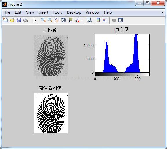
%计算全局阈值
clc;
clear all;
close all;
f=imread('0.tif');
figure;imshow(f);title('原图像');	%显示原图像
%%
%全局阈值分割
count=0;
T=mean2(f);
done=false;
while ~done
    count=count+1;
    g=f>T;
    Tnext=0.5*(mean(f(g))+mean(f(~g)));
    done=abs(T-Tnext)<0.5;
    T=Tnext;
end
disp('count的值为:');
disp(['count=',num2str(count)])  %打印输出count的值
disp('T的值为:');
disp(['T=',num2str(T)])       %打印输出T的值
g=im2bw(f,T/255);
figure;subplot(2,2,1);imshow(f);title('原图像');
subplot(2,2,2);imhist(f);title('f直方图');
subplot(2,2,3);imshow(g);title('阈值后图像');
(3)结果
2、使用边缘改进全局阈值处理
(1)步骤
(1) 用任何方法计算来自f (x,y)的边缘图像。边缘图像可以是梯度或拉普拉斯的绝对值。
(2) 指定阈值T。
(3) 用来自步骤(2)的阈值对来自步骤(1)的图像进行阈值处理,产生一副二值图像gT(x,y)。这幅图像在步骤(4)中选择来自f (x,y)的对应于强边缘的像素并作为标记图像使用。
(4) 仅用f (x,y)中的像素计算直方图,对应gT(x,y)中1 值像素的位置。
(5) 用来自步骤(4)中的直方图,通过全局阈值方法(如Otsu's 方法)来分割f (x,y)。
通常,通过指定T 值(T 值与某个百分比对应)来典型地设置高值(例如90%),因此,在阈值计算中使用图像的边缘上没有多少像素。自定义函数percentile2i可用于这个目的。该函数计算灰度值I,I 对应指定的百分比。语法是:
I = percentile2i(h, P)
其中,h 是图像的直方图,p 是在[0, 1]范围内的百分比值。输出I 是灰度级(也在[0, 1]范围内),对应第p 个百分点。
(2)代码
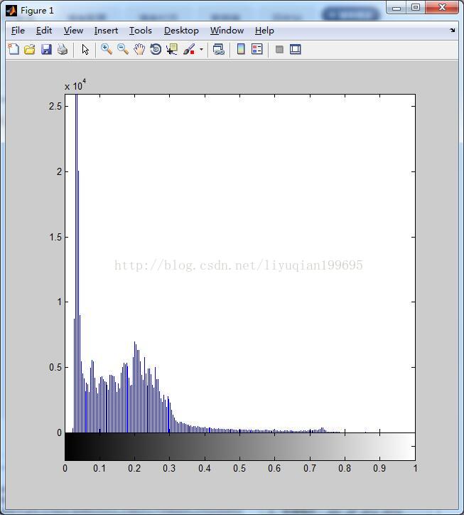
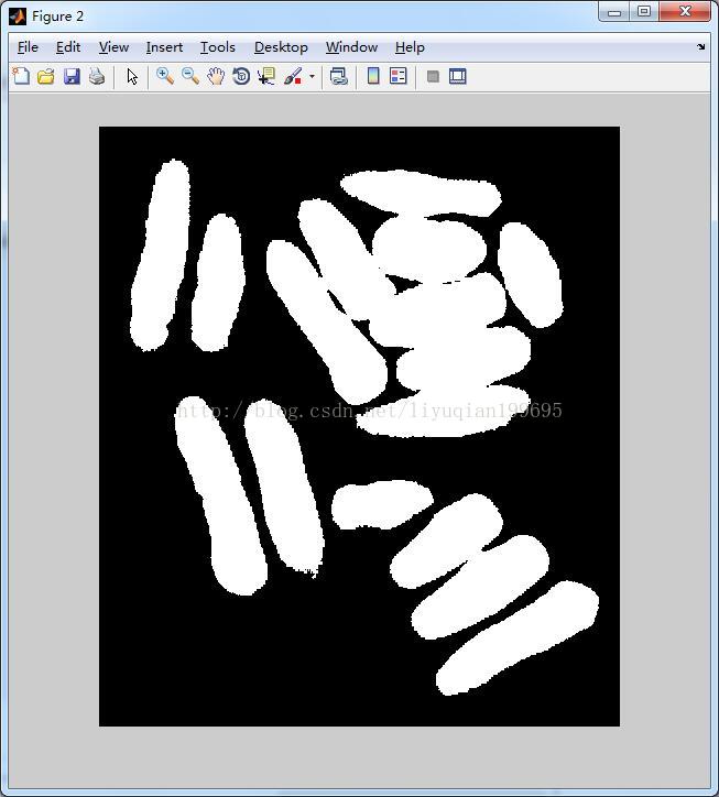
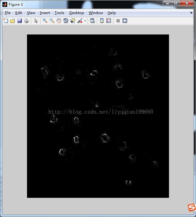
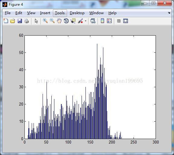
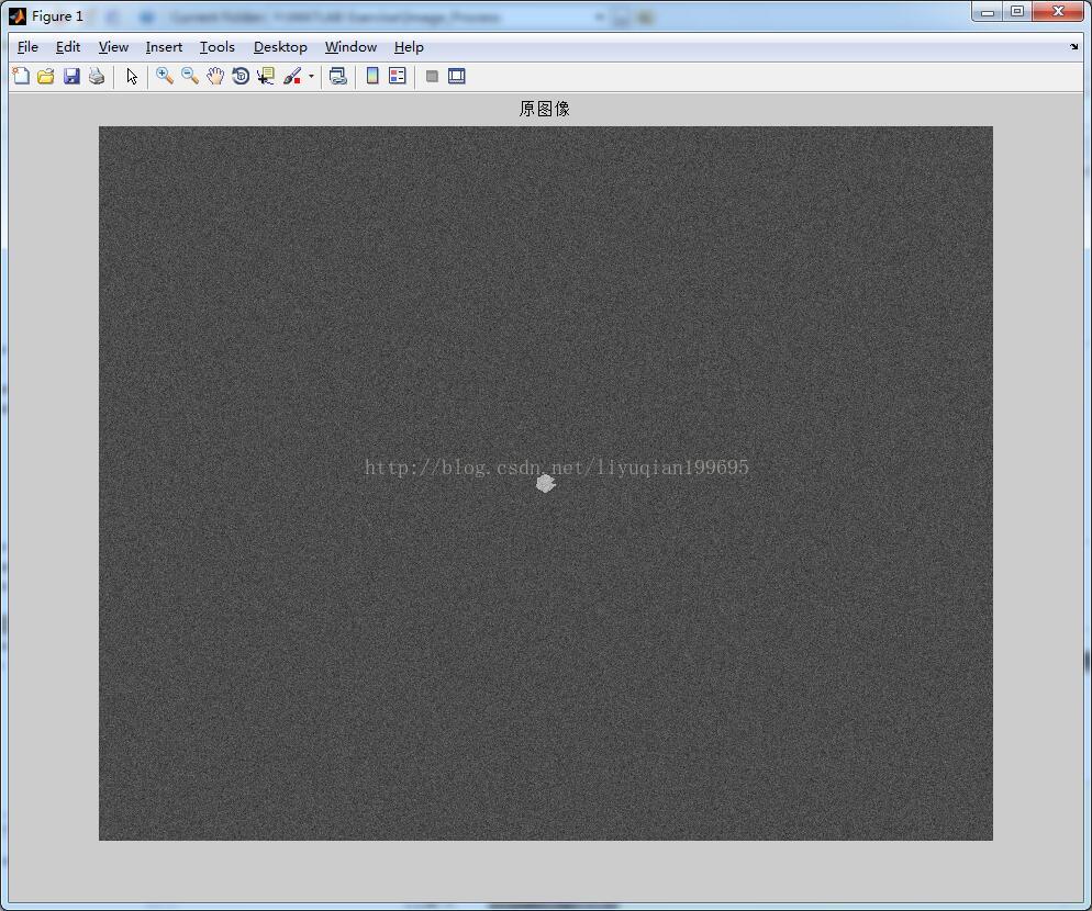
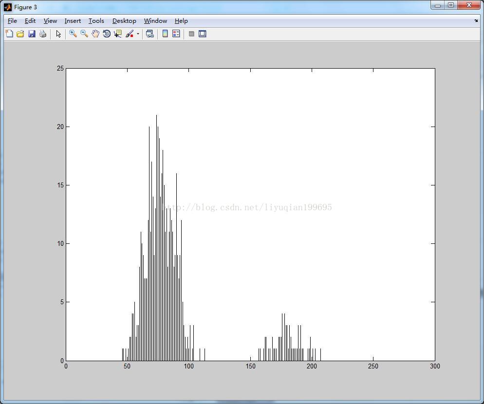
%计算全局阈值
clc;
clear all;
close all;
src=imread('a.tif');
figure;imshow(src);title('原图像');%显示原图像
%%
%计算梯度
f = tofloat(src);
sx = fspecial('sobel');
sy = sx';
gx = imfilter(f,sx,'replicate');
gy = imfilter(f,sy,'replicate');
grad = sqrt(gx.*gx + gy.*gy);
grad = grad/max(grad(:));
%%
%得到grad 的直方图,并使用高的百分比(99.9%)估计梯度的阈值
h = imhist(grad);
Q = percentile2i(h, 0.999);
%%
%用Q 对梯度做阈值处理,形成标记图像,并且从f 中提取梯度值比Q大的点,得到结果的直方图:
markerImage = grad > Q;
figure, imshow(markerImage) % Fig. 10.16(c).
fp = f.*markerImage;
figure, imshow(fp) % Fig. 10.16(d).
hp = imhist(fp);
%%
%用结果的直方图得到Otsu 阈值
hp(1) = 0;
bar(hp, 0) % Fig. 10.16(e).
T = otsuthresh(hp);
T*(numel(hp) - 1)
g = im2bw(f, T);
figure, imshow(g)
函数percentile2i定义
function I=percentile2i(h,P)
%PERCENTILE2I Computes an intensity value given a percentile.
% I=PERCENTILE2I(H,P) Given a percentile ,p,and a histogram,
% H, this function computes an intensity ,I representing
% the Pth percentile and returns the value  in I. P must be in the
% range [0,1] and I is returned as a value in the range [0,1] also.
% Example:
% I=percentile2i(h,0.5)

% Check value of P
if P<0 || P>1
    error('The percentile must be in the range [0,1].');
end

% Normalized the histogram to unit area.if it is already normalized
% the following computation has no effect.
h=h/sum(h);

% Camulative distribution
C=cumsum(h);
% Calculations.
idx=find(C >= P,1,'first');
% Subtract 1 from idx because indexing starts at 1,but intensities
% start at 0. Also ,normalize to the range [0,1].
I=(idx-1)/(numel(h)-1);
函数otsuthresh定义
function [T, SM] = otsuthresh(h)
%OTSUTHRESH Otsu's optimum threshold given a histogram.
% [T, SM] = OTSUTHRESH(H) computes an optimum threshold, T, in the
% range [0 1] using Otsu's method for a given a histogram, H.
% Normalize the histogram to unit area. If h is already normalized,
% the following operation has no effect.
h = h/sum(h);
h = h(:); % h must be a column vector for processing below.
% All the possible intensities represented in the histogram (256 for
% 8 bits). (i must be a column vector for processing below.)
i = (1:numel(h))';
% Values of P1 for all values of k.
P1 = cumsum(h);
% Values of the mean for all values of k.
m = cumsum(i.*h);
% The image mean.
mG = m(end);
% The between-class variance.
sigSquared = ((mG*P1 - m).^2)./(P1.*(1 - P1) + eps);
% Find the maximum of sigSquared. The index where the max occurs is
% the optimum threshold. There may be several contiguous max values.
% Average them to obtain the final threshold.
maxSigsq = max(sigSquared);
T = mean(find(sigSquared == maxSigsq));
% Normalized to range [0 1]. 1 is subtracted because MATLAB indexing
% starts at 1, but image intensities start at 0.
T = (T - 1)/(numel(h) - 1);
% Separability measure.
SM = maxSigsq / (sum(((i - mG).^2) .* h) + eps);
(3)结果

3、用拉普拉斯边缘信息改进全局阈值处理
(1)代码
%
clc;
clear all;
close all;
src=imread('b.tif');
figure;imshow(src);title('原图像');%显示原图像
%%
%
f = tofloat(src);
imhist(f) 		% 图像直方图
hf = imhist(f);
[Tf SMf] = graythresh(f);
gf = im2bw(f, Tf);
figure, imshow(gf) 	% 显示阈值图像.
%%
w = [-1 -1 -1; -1 8 -1; -1 -1 -1];
lap = abs(imfilter(f, w, 'replicate'));
lap = lap/max(lap(:));
h = imhist(lap);
Q = percentile2i(h, 0.995);
markerImage = lap > Q;
fp = f.*markerImage;
figure, imshow(fp) %
hp = imhist(fp);
hp(1) = 0;
figure, bar(hp, 0) %
T = otsuthresh(hp);
g = im2bw(f, T);
figure, imshow(g) %
(2)结果