李宏毅学习笔记35.GAN.06.Tips for Improving GAN

简介

Martin Arjovsky, Soumith Chintala, Leon Bottou, Wasserstein GAN, arXiv prepring, 2017
Ishaan Gulrajani, Faruk Ahmed,Martin Arjovsky, Vincent Dumoulin, Aaron Courville, “Improved Training of Wasserstein GANs”,arXiv prepring,2017
这节讲GAN的优化。
公式输入请参考：在线Latex公式

JS divergence来衡量分布的问题

JS divergence is not suitable. 原因在于：
In most cases, $P_G$ and $P_{data}$ are not overlapped.
就是生成的数据和真实数据是不重叠的。不重叠有两方面的原因：
1、数据本身的问题The nature of data
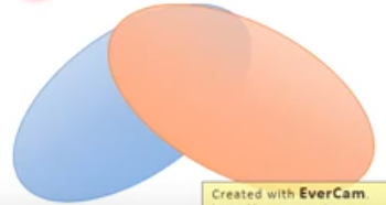
Both $P_{data}$ and $P_G$ are low-dim manifold in high-dim space.The overlap can be ignored.
例如：图片是高（三）维空间中的低（二）维空间的manifold。
如下图所示，可以看到两个曲线overlap的部分是很小的。

2、采样Sampling的原因
尽管数据本来是有overlap，但是我们不是取所有的数据：
Even though $P_{data}$ and $P_G$ have overlap.

我们是对这两堆分布进行采样，我们不会采样全部，而是部分：

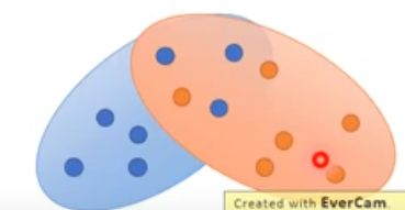
以上两个分布采样的结果是不会有overlap的，除非你采样超多点，因此这两个采样结果可以看做是两个不同的分布：

也就是说If you do not have enough sampling ……结果就是没有重合。
没有重合的时候，用JS divergence来衡量分布，会发生什么？

What is the problem of JS divergence?

只要两个分布不重合，那么算出来的结果都一样： $log2$
JS divergence is $log2$ if two distributions do not overlap

按理说 $P_{G_1}$要比 $P_{G_0}$好，因为它比 $P_{G_0}$要更加接近 $P_{data}$，JS divergence都一样，除非二者重合，两个才会有JS divergence=0。这样在不重合的状态下是没有办法做优化（train）的。
结果为什么会是： $log2$？
Intuition: If two distributions do not overlap, binary classifier achieves 100% accuracy.
用一个二分类的分类器对不重叠的两个分布做分类，总是可以得到100%的准确率，因此其cost都是一样的。
Same objective value is obtained. →Same divergence.
因此在GAN中用二分类来训练是很难收敛的。例如：
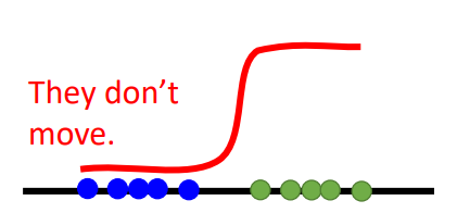
用绿色点代表真实数据
蓝色点代表生成数据
如果是一个sigmoid函数的话，可以看到蓝色点这块的梯度都是0，所以在GD的时候是不会更新（动）的。所以有人提出说，不要把这个分类函数训练得太好，使得整个分类函数在蓝色点部分有梯度，这样才可以进行梯度更新，但是这个训练得好不好（太用力，没梯度，不够用力，discriminator无法工作），很难把握。

因此为了做GAN的优化，出现了LSGAN

Least Square GAN (LSGAN)

算法思想就是用线性分类器替换sigmoid分类器。也就是把分类问题换成了回归问题。
Replace sigmoid with linear (replace classification with regression)

train的目标是使得真实数据越接近1越好，生成数据越接近0越好。

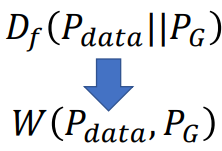
Wasserstein GAN (WGAN): Earth Mover’s Distance

Wasserstein中a发[æ]的音，思想就是不用JS divergence来衡量两个分布的差别，而是用另外一个方法：Earth Mover’s Distance。这个玩意的概念很土。。。
把P和Q看作是两堆土，而你是蓝翔毕业的挖掘机(Earth Mover)司机，要把P这堆土（原文是挖到Q那里，但是应该不是这个意思）挖成Q的形状，而Earth Mover’s Distance就是挖掘机来回移动的平均距离。
• Considering one distribution P as a pile of earth, and another distribution Q as the target
• The average distance the earth mover has to move the earth.

上面的分布是简化了的，土堆应该是这样：

要把P变成Q，可以有很多种挖法：

上图中的左边是是把邻近的土进行移动，右边是比较远的土进行移动。我们一般用左边的那种。
There many possible “moving plans”.
Using the “moving plan” with the smallest average distance to define the earth mover’s distance.
Best “moving plans” of this example

正式的定义：
A “moving plan” is a matrix. The value of the element is the amount of earth from one position to another.
Average distance of a plan $\gamma$:
$B(\gamma)=\sum_{x_p,x_q}\gamma(x_p,x_q)||x_p-x_q||$
Earth Mover’s Distance:
$W(P,Q)=\underset{\gamma\in\prod}{min}B(\gamma)$
这个矩阵中某个点(x,y)代表从行x移动多少土到列y，这个点的颜色越亮，那么代表移动的土越多。
行x所有点加起来，对应P中对应第x堆土；
列y所有点加起来，对应Q中对应第y堆土。
给定矩阵（确定移动方案后） $\gamma$，计算移动距离 $B(\gamma)$，如上面公式所示，然后穷举所有移动方案，找到最小那个。

也就是说这个方法要接一个优化方案后才能得到解。

Why Earth Mover’s Distance?

用Earth Mover’s Distance来替换JS divergence

那么也就改善了之前两个分布不重叠无法更新梯度的缺点：

可以看到d50比d0是有进步的，所以梯度才能不断更新迭代，最后到达两个分布距离为0的目标。

WGAN

如何用wasserstein distance来衡量两个分布，这个过程的证明比较复杂，直接给结论：
Evaluate wasserstein distance between $P_{data}$ and $P_G$
$V(G,D)=\underset{D\in 1-Lipschitz}{max}\{E_{x\sim P_{data}}[D(x)]-E_{x\sim P_{G}}[D(x)]\}$
公式的意思是：如果x是从 $P_{data}$ 采样出来的，希望他的Discriminator值越大越好，如果是从 $P_G$采样出来的，希望他的Discriminator值越小越好，另外还有一个约束就是D要是一个 $1-Lipschitz$的函数（啥意思后面讲，就是要D越平滑越好）
为什么要平滑呢，如果没有平滑的这个限制：

D就会在生成数据 $P_{data}$的地方趋向于负无穷大，在真实数据 $P_G$的地方趋向于正无穷大。两个分布就会差很多。加入平滑限制，会使得D不会无限的上升和下降，会停在某个地方。

---

$Lipschitz\space Function$
$||f(x_1)-f(x_2)||\leq K||x_1-x_2||$
可以看到公式左边是输出的变化，右边是输入的变化，也就是说输出的变化要小于K倍的输入的变化。
当K=1，我们就把这个满足这个不等式的函数称为 $1-Lipschitz$
也就是
$||f(x_1)-f(x_2)||\leq ||x_1-x_2||$
也就是不会变化很快。例如下面的绿色函数比较像 $1-Lipschitz\space Function$，蓝色函数就肯定不是 $1-Lipschitz\space Function$

---

如何满足 $1-Lipschitz\space Function$约束条件呢？原论文使用的方法是：Weight Clipping
Force the parameters $w$ between $c$ and $-c$. After parameter update,
if w > c, w = c;
if w < -c, w = -c
这个方法很简单，其实用这个方法弄出来的函数并不满足 $1-Lipschitz\space Function$约束条件，但是基本能work，能达到使得D平滑的目的。也是没有办法的办法，因为 $1-Lipschitz\space Function$不好优化。

Improved WGAN (WGAN-GP)

对Weight Clipping进行改进，函数还是一样：
$V(G,D)=\underset{D\in 1-Lipschitz}{max}\{E_{x\sim P_{data}}[D(x)]-E_{x\sim P_{G}}[D(x)]\}$
但是Improved WGAN对于约束换了一个角度，就是梯度的norm要小于等于1。
A differentiable function is 1-Lipschitz if and only if it has gradients with norm less than or equal to 1 everywhere.
这个转换和之前的约束是一样的。

关于norm的计算是有一个近似计算的方法的：
$V(G,D)\approx\underset{D}{max}\{E_{x\sim P_{data}}[D(x)]-E_{x\sim P_{G}}[D(x)]-\lambda\int_xmax(0,||\triangledown _xD(x)||-1)dx\}$
后面这个积分项类似于正则项，它的作用是对所有的x做积分，然后取一个max，这个max的意思当Discriminator的梯度的norm大于1，那么就会存在正则项，如果Discriminator的梯度的norm小于1，那么这项为0，没有正则项（不惩罚）。但是这样会有问题，我们不可能对所有高维空间中的x都进行求积分这个操作，我们的x是sample出来的。因此再次把正则项进行近似：
$-\lambda E_{x\sim P_{penalty}}[max(0,||\triangledown _xD(x)||-1)]$
这个正则项保证所有采样出来的x满足Discriminator的梯度的norm小于1
把这个惩罚项拿出来，做一个可视化，实际上这个penalty项就是从 $P_{data}$ 中随便取一点，然后从 $P_G$中随便取一点，然后在这两点的连线上进行采样，得到 $x\sim penalty$

把这些sample到的 $x\sim penalty$范围画出来就是上面的蓝色部分，为什么不是对整个空间中的x都做penalty呢？原文说实验结果表明这样做结果比较好。。。
“Given that enforcing the Lipschitz constraint everywhere is intractable, enforcing it only along these straight lines seems sufficient and experimentally results in good performance.”
从另外一个方面来看， $P_G$要沿着梯度的方向向 $P_{data}$ 靠近，靠近移动的方向就是蓝色区域，其他区域也不会去，所以这样解释也可以。
Only give gradient constraint to the region between $P_{data}$ and $P_G$ because they influence how $P_G$ moves to $P_{data}$.
再来一个trick，之前说近似后的约束是希望梯度大于1就会有惩罚，小于1不会有惩罚（ $max(0,||\triangledown _xD(x)||-1)$这里。）但是在实作的时候，用的正则项为： $(||\triangledown _xD(x)||-1)^2$，意思是希望梯度越接近1越好。原文：
“Simply penalizing overly large gradients also works in theory, but experimentally we found that this approach converged faster and to better optima.”
理由就是实作上效果好。。。
当然这个方法也有缺点，它的penalty的点是从两个分布中随机选点然后连接，然后做采样，如果有下图的两个分布明显这样做有问题：

选择红色那个点是不好的，（因为黄色的点移动也是移动到黑色点那个位置，也就是以黑色点为目标，而不是以红色点为目标。）应该选下图中黑色的点的连线来做采样比较合适。但是找黑色的点又比较麻烦。。。

后来又研究者对Improved WGAN提出Improved Improved WGAN算法，改进的地方在于把penalty放在了 $P_{data}$的范围。

Spectrum Norm

上面讲的WGAN比较弱，一来都是用近似的方法搞的，解释不通就说反正实作就是这样；二来只有在某个区域Discriminator的norm才会满足小于1的条件。Spectrum Norm就直接，所有范围的x经过Discriminator后的norm都会满足小于1的条件。（不展开）
Spectral Normalization → Keep gradient norm smaller than 1 everywhere [Miyato, et al., ICLR, 2018]
下面是生成狗狗的DEMO，原文是动图。。。

GAN to WGAN（如何将GAN的算法改为WGAN的算法）

Algorithm of GAN（Review）

Initialize $\theta_d$ for $D$ and $\theta_g$ for $G$.
• In each training iteration:

---

这块分割线内是训练Discriminator，重复k次，这里一定要训练到收敛为止，目的是找到 $\underset{D}{\text{max}}V(G,D)$（实作的时候一般没有办法真的训练到收敛或者卡在局部最小点，因此这里找到的是 $\underset{D}{\text{max}}V(G,D)$的lower bound）。
••Sample m examples $\{x^1,x^2,\cdots,x^m\}$ from data distribution $P_{data}(x)$.（找到真实对象）
••Sample m noise examples $\{z^1,z^2,\cdots,z^m\}$ from the prior $P_{prior}(z)$.（这个先验分布种类不是很重要）
•••Obtaining generated data $\{\tilde x^1,\tilde x^2,\cdots,\tilde x^m\},\tilde x^i=G(z^i)$.（找到生成对象）
•• Update discriminator parameters $\theta_d$ to maximize
$\tilde V=\cfrac{1}{m}\sum_{i=1}^mlogD(x^i)+\cfrac{1}{m}\sum_{i=1}^mlog(1-D(\tilde x^i))\tag1$
$\theta_d\leftarrow\theta_d+\eta\triangledown\tilde V(\theta_d)$

---

---

这块分割线内是训练Generator，重复1次，目的是减少JSD
••Sample another m noise samples $\{z^1,z^2,\cdots,z^m\}$ from the prior $P_{prior}(z)$
••Update generator parameters $\theta_g$ to minimize
$\tilde V=\cfrac{1}{m}\sum_{i=1}^mlogD(x^i)+\cfrac{1}{m}\sum_{i=1}^mlog(1-D(G(z^i)))\\ \theta_g\leftarrow\theta_g-\eta\triangledown\tilde V(\theta_g)$
由于 $\cfrac{1}{m}\sum_{i=1}^mlogD(x^i)$和 $G$函数无关，所以在求最小值的时候可以忽略：
$\tilde V=\cfrac{1}{m}\sum_{i=1}^mlog(1-D(G(z^i)))\tag2$
$\theta_g\leftarrow\theta_g-\eta\triangledown\tilde V(\theta_g)$

---

Algorithm of WGAN

把原始GAN算法中的公式1和公式2进行修改，具体如下：
对于公式1（训练discriminator），实际上就是把sigmoid函数去掉，变成：
$\tilde V=\cfrac{1}{m}\sum_{i=1}^mD(x^i)-\cfrac{1}{m}\sum_{i=1}^mD(\tilde x^i)\tag3$
当然在训练discriminator的时候要注意使用Weight clipping /Gradient Penalty …等技巧，否则很难收敛。
对于公式2（训练generator），改为：
$\tilde V=-\cfrac{1}{m}\sum_{i=1}^mD(G(z^i))$

Energy-based GAN (EBGAN)

Junbo Zhao, et al., arXiv, 2016
这个算法还有一个变形，不展开，大概看看这个算法。
大概思想就是Generator不变，用autoencoder来做Discriminator。
Using an autoencoder as discriminator D.
计算过程如下图所示：

生成的图片进入粉色部分（Discriminator），先经过一个Autoencoder，还原后，计算出还原图像和原图的reconstruction error（上图中是0.1），然后乘上一个 -1，得到Discriminator的输出（上例中是-0.1）
所以从整体上来看Discriminator和之前的GAN的Discriminator一样，输入一个对象，得到这个对象和真实对象的差距，只不过是得到这个差距的方法不一样，之前是JS divergence，这里是Autoencoder。简单来说就是根据一个图片是否能够被reconstruction，如果能被还原得很好，说明这个图片是一个high quality的图片，反之亦然。
这个方法的好处就是Autoencoder是可以pretrain的，不需要negative example来训练，直接给它positive example来minimize reconstruction error即可。
➢Using the negative reconstruction error of auto-encoder to determine the goodness.
➢Benefit: The auto-encoder can be pre-train by real images without generator.
这样还有一个好处，原来的GAN刚开始训练的时候generator和discriminator都很弱，要不断迭代后discriminator才随着generator的变强而变强，这个方法discriminator不依赖generator，直接开局就很强。
EBGAN在训练的时候有一个trick，如果只是希望生成图片（蓝色）的分数，即reconstruction error越大越好（取负号后变小），那么会让autoencoder训练出来直接输出noise，因为Hard to reconstruct, easy to destroy，要得到低分很简单，只要输出noise，就会得到reconstruction error超级大（取负号后变小），这样训练出来的discriminator不是我们想要的。

因此我们会在训练的过程中为reconstruction error（取负号后）添加一个margin下限（超参数），让reconstruction error（取负号后）小到一定程度即可。

Outlook: Loss-sensitive GAN (LSGAN)

这个GAN也用到了margin的概念，之前的WGAN，Discriminator是希望真实数据得分越大越好，生成数据得分越小越好

但是有些生成数据已经比较真实了，没有必要要搞得很小。例如：下图中的 $x''$比较接近真实数据 $x$，即 $\Delta(x,x'')$比较小， $x'$没有那么接近真实数据 $x$，即 $\Delta(x,x')$比较大，可以看到 $\Delta(x,x')$的margin压得比较小，而 $\Delta(x,x'')$的margin比较大。

Reference

• Ian J. Goodfellow, Jean Pouget-Abadie, Mehdi Mirza, Bing Xu, David WardeFarley, Sherjil Ozair, Aaron Courville, Yoshua Bengio, Generative Adversarial Networks, NIPS, 2014
• Sebastian Nowozin, Botond Cseke, Ryota Tomioka, “f-GAN: Training Generative Neural Samplers using Variational Divergence Minimization”, NIPS, 2016
• Martin Arjovsky, Soumith Chintala, Léon Bottou, Wasserstein GAN, arXiv, 2017
• Ishaan Gulrajani, Faruk Ahmed, Martin Arjovsky, Vincent Dumoulin, Aaron Courville, Improved Training of Wasserstein GANs, NIPS, 2017
• Junbo Zhao, Michael Mathieu, Yann LeCun, Energy-based Generative Adversarial Network, arXiv, 2016
• Mario Lucic, Karol Kurach, Marcin Michalski, Sylvain Gelly, Olivier Bousquet, “Are GANs Created Equal? A Large-Scale Study”, arXiv, 2017
• Tim Salimans, Ian Goodfellow, Wojciech Zaremba, Vicki Cheung, Alec Radford, Xi Chen Improved Techniques for Training GANs, NIPS, 2016
• Martin Heusel, Hubert Ramsauer, Thomas Unterthiner, Bernhard Nessler, Sepp Hochreiter, GANs Trained by a Two Time-Scale Update Rule Converge to a Local Nash Equilibrium, NIPS, 2017
• Naveen Kodali, Jacob Abernethy, James Hays, Zsolt Kira, “On Convergence and Stability of GANs”, arXiv, 2017
• Xiang Wei, Boqing Gong, Zixia Liu, Wei Lu, Liqiang Wang, Improving the Improved Training of Wasserstein GANs: A Consistency Term and Its Dual Effect, ICLR, 2018
• Takeru Miyato, Toshiki Kataoka, Masanori Koyama, Yuichi Yoshida, Spectral Normalization for Generative Adversarial Networks, ICLR, 2018