NLP基础概览 + Spell Correction with Noisy Channel

往期文章链接目录

NLP = NLU + NLG

• NLU: Natural Language Understanding
• NLG: Natural Language Generation

NLG may be viewed as the opposite of NLU: whereas in NLU, the system needs to disambiguate the input sentence to produce the machine representation language, in NLG the system needs to make decisions about how to put a concept into human understandable words.

Classical applications in NLP

• Question Answering

• Sentiment Analysis

• Machine Translation

• Text Summarization: Text summarization refers to the technique of shortening long pieces of text. The intention is to create a coherent and fluent summary having only the main points outlined in the document. It involves both NLU and NLG. It requires the machine to first understand human text and overcome the long distance dependence problems (NLU) and then generate human understandable text (NLG).

  • Extraction-based summarization: The extractive text summarization technique involves pulling keyphrases from the source document and combining them to make a summary. The extraction is made according to the defined metric without making any changes to the texts. The grammar might not be right.
  • Abstraction-based summarization: The abstraction technique entails paraphrasing and shortening parts of the source document. The abstractive text summarization algorithms create new phrases and sentences that relay the most useful information from the original text — just like humans do.
  • Therefore, abstraction performs better than extraction. However, the text summarization algorithms required to do abstraction are more difficult to develop; that’s why the use of extraction is still popular.

• Information Extraction: Information extraction is the task of automatically extracting structured information from unstructured and/or semi-structured machine-readable documents and other electronically represented sources. QA uses information extraction a lot.

• Dialogue System

  • task-oriented dialogue system.

Text preprocessing

Tokenization

For Chinese, classical methods are forward max-matching and backward max-matching.

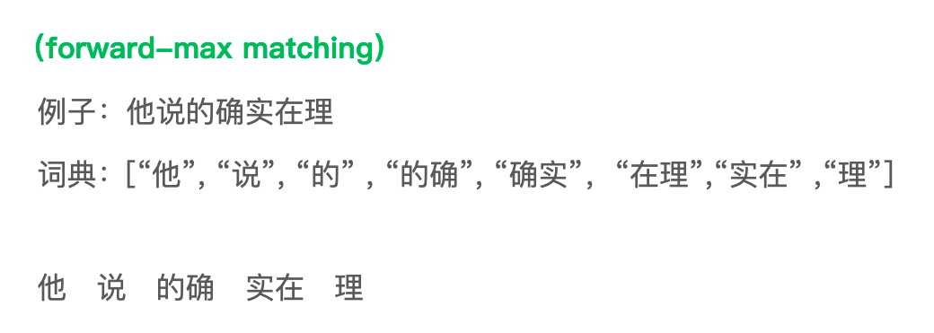
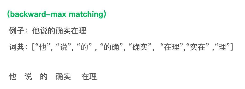
Shortcoming: Do not take semantic meaning into account.

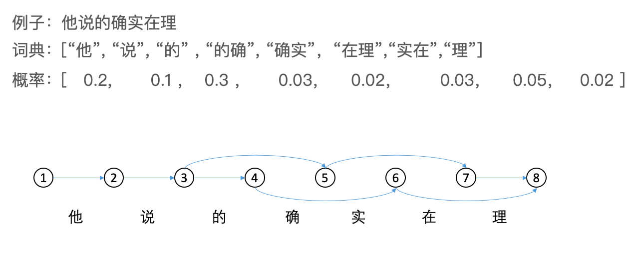
Tokenization based on Language Modeling. Given an input, generate all possible way to split the sentence and then find the one with the highest possibility.

Unigram model:
$P(s) = P(w_1)P(w_2)...P(w_k)$

Bigram model:
$P(s) = P(w_1)P(w_2 | w_1)P(w_3|w_2) ... P(w_k |w_{k-1})$

Alternative: Use Viterbi algorithm (Dynamic Programming) to find the optimal way of splitting. Every directed graph path corresponds to a way to split a sentence.

• Spell Correction

  • Way 1: Go through the vocabulary and then return the words with the smallest edit distance.

  • Way 2: Generate all strings with edit distance 1 or 2, then filter and return (faster than Way 1). We will discuss how to filter at the end of the summary and the filtering method we introduce is called Noisy Channel model.

Lowercasing

Lowercasing text data is one of the simplest and most effective form of text preprocessing. It can help in cases where your dataset is not very large and thus solve the sparsity issue.

Stop-word removal

The intuition behind using stop words is that, by removing low information words from text, we can focus on the important words instead. Think about it as a feature selection process. In general, we won’t do stop-word removal when dealing with machine translation.

Zipf’s law: Zipf’s law is an empirical law refers to the fact that many types of data studied can be approximated with a Zipfian distribution. It states that given some corpus, the frequency of any word is inversely proportional to its rank in the frequency table. Thus the most frequent word will occur approximately twice as often as the second most frequent word, three times as often as the third most frequent word.

Normalization

Text normalization is the process of transforming text into a standard form. For example, the word “gooood” and “gud” can be transformed to “good”. Another example is mapping of near identical words such as “stopwords”, “stop-words” and “stop words” to just “stopwords”. Text normalization is important for noisy texts such as social media comments, text messages and comments to blog posts where abbreviations, misspellings and use of out-of-vocabulary words (oov) are prevalent.

Two popular ways to normalizr are Stemming & Lemmatization.

The goal of both stemming and lemmatization is to reduce inflectional forms and sometimes derivationally related forms of a word to a common base form.

However, the two words differ in their flavor. Stemming usually refers to a crude heuristic process that chops off the ends of words in the hope of achieving this goal correctly most of the time, and often includes the removal of derivational affixes. Lemmatization usually refers to doing things properly with the use of a vocabulary and morphological analysis of words, normally aiming to remove inflectional endings only and to return the base or dictionary form of a word, which is known as the lemma.

TF-IDF

TF-IDF works by increasing proportionally to the number of times a word appears in a document, but is offset by the number of documents that contain the word. So, words that are common in every document, such as this, what, and if, rank low even though they may appear many times, since they don’t mean much to that document in particular. However, if a word appears many times in a document, while not appearing many times in others, it probably means that it’s very relevant.

Formula

There are multiple ways to caluculate. Here is one: the TF-IDF score for each word $w$ in the document $d$ from the document set $D$ is calculated as follows:

$tf\text{-}idf \, (w,d,D) = tf \, (w,d) \cdot idf \, (w,D)$

where

$tf \, (w,d) = \text{freq} \, (w,d) \\ idf \,(w, D) = \log \frac{|D|}{N(w)}$

where $\text{freq} \, (w,d)$ is the frequency of word $w$ in the document $d$. $|D|$ is the number of document and $N(w)$ is the number of documents having word $w$. Therefore we have a TF-IDF representation for all words in all documents. Note that in every document, the number of word is equal to the number of TF-IDF representation.

Ways to compute similarities between sentences

Common ways are using Dot Product, Cosine Similarity, Minkowski distance, and Euclidean distance.

Dot Product: $d(x,y) = \langle x, y\rangle$

Cosine Similarity: $d(x, y) = \frac{\langle x, y\rangle}{\|x\|\|y\|}$

Euclidean distance (squared): $d(x, y) = \|x-y\|^2 = \|x\|^2 +\|y\|^2 - 2\langle x , y\rangle$

Minkowski distance: $d(x, y) = (\sum_{i=1}^n |x_i - y_i|^p ) ^ \frac{1}{p}$

Comparision between Cosine Similarity and Euclidean distance:

• In general, the Cosine Similarity removes the effect of document length. For example, a postcard and a full-length book may be about the same topic, but will likely be quite far apart in pure “term frequency” space using the Euclidean distance. However,tThey will be right on top of each other in cosine similarity.

• Euclidean distance mainly measures the numeric difference between $x$ and $y$. Cosine Similarity mainly measures the difference of direction between $x$ and $y$.

• However, if we normalize x and y, the two calculations are equivalent. If we assume $x$ and $y$ are normalized, then Cosine Similarity is $\langle x , y\rangle$, and Euclidean distance (squared) is $2(1 - \langle x , y\rangle)$. As you can see, minimizing (square) euclidean distance is equivalent to maximizing cosine similarity if the vectors are normalized.

Noisy Channel model ( for spell correction)

Intuition:

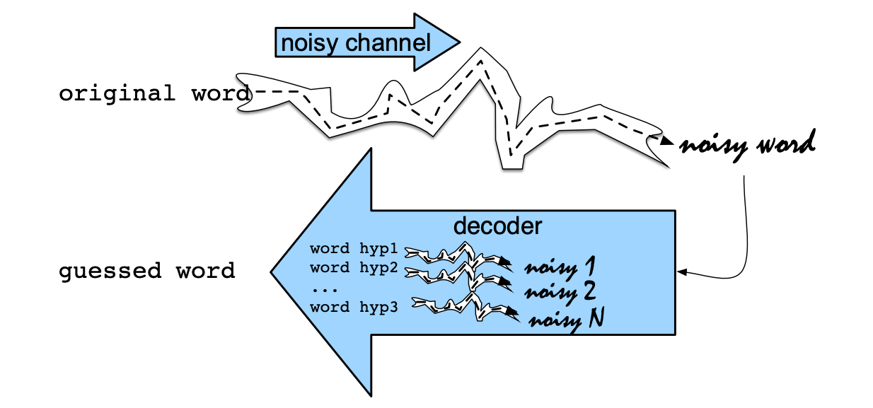
The intuition of the noisy channel model is to treat the misspelled
word as if a correctly spelled word had been “distorted” by being passed through a
noisy communication channel. This channel introduces noise, making it hard to recognize the true word. Our goal is to find the true word by passing every word of the language through our model of the noisy channel and seeing which one comes the closest to the misspelled word.

Process:

We see an observation $x$ (a misspelled word) and our job is to find the word $w$ that generated this misspelled word. Out of all possible words in the vocabulary $V$ we want to find the word $w$ such that $P(w|x)$ is highest. So our objective function is $\mathop{\rm argmax}\limits_{w \, \in \, V} P(w|x)$

We can re-write our objective function as $\mathop{\rm argmax}\limits_{w \, \in \, V} \frac{P(x|w)P(w)}{p(x)}$

Since $P(x)$ doesn’t change for each choice of word $w$, we can drop it and simplify the objective function as

$\mathop{\rm argmax}\limits_{w \, \in \, V} P(x|w)P(w)$

The channel model (or likelihood) of the noisy channel producing any particular observation sequence x is modeled by $P(x|w)$. The prior probability of a hidden word is modeled by $P(w)$. We can compute the most probable word $\hat w$ given that we’ve seen some observed misspelling $x$ by multiplying the prior $P(w)$ and the likelihood $P(x|w)$ and choosing the word for which this product is greatest.

We apply the noisy channel approach to correcting non-word spelling errors by
taking any word not in our spelling dictionary, generating a list of candidate words,
ranking them according to the objective function defined above and then picking the highest-ranked one. In fact, we can modify the objective function to refer to this list of candidate words instead of the full vocabulary $V$ as follows:

To find this list of candidates we’ll use the Minimum Edit Distance algorithm. Note that the types of edits are:

• Insertion
• Deletion
• Substitution
• Transposition of two adjacent letters (perticular in tasks like spell correction)

why we prefer not to compute $p(w|x)$ directly?

• Two distributions $p(x|w)$ and $p(w)$ (the language model) can be estimated seperately.

• If we compute $p(w|x)$ directly, that means we just find a word that maximize the probability $p(w|x)$ but do not put the word in the context (surrounding words). Thus the accuracy of the spell correction is pretty low.

• On the other hand, it’s worth noting that the surrounding words will make the choice of word clearer. If we maximize $P(x|w)P(w)$, there is a prior term $P(w)$ which we can use bigram, trigram, etc, to compute. Usually, bigram, trigram are better than unigram since they take surrounding words into account.

How to compute channel model $P(x|w)$

A perfect model of the probability that a word will be mistyped would condition on all sorts of factors: who the typist was, whether the typist was left-handed or right-handed, and so on. Luckily, we can get a pretty reasonable estimate of $P(x|w)$ just by looking at local context: the identity of the correct letter itself, the misspelling, and the surrounding letters. For example, the letters $m$ and $n$ are often substituted for each other; this is partly a fact about their identity (these two letters are pronounced similarly and they are next to each other on the keyboard) and partly a fact about context (because they are pronounced similarly and they occur in similar contexts). For more detail about how to compute $P(x|w)$, check out https://web.stanford.edu/~jurafsky/slp3/B.pdf.

---

Reference:

• https://en.wikipedia.org/wiki/Natural-language_generation
• https://towardsdatascience.com/a-quick-introduction-to-text-summarization-in-machine-learning-3d27ccf18a9f
• https://en.wikipedia.org/wiki/Information_extraction
• https://kavita-ganesan.com/text-preprocessing-tutorial/
• https://web.stanford.edu/~jurafsky/slp3/B.pdf
• https://en.wikipedia.org/wiki/Zipf%27s_law
• https://stackoverflow.com/questions/1787110/what-is-the-difference-between-lemmatization-vs-stemming
• https://monkeylearn.com/blog/what-is-tf-idf/
• https://www.jianshu.com/p/4f0ee6d023a5
• https://www.reddit.com/r/MachineLearning/comments/493exs/why_do_they_use_cosine_distance_over_euclidean/
• https://stats.stackexchange.com/questions/72978/vector-space-model-cosine-similarity-vs-euclidean-distance
• https://datascience.stackexchange.com/questions/6506/shall-i-use-the-euclidean-distance-or-the-cosine-similarity-to-compute-the-seman
• https://www.quora.com/Natural-Language-Processing-What-is-a-noisy-channel-model

往期文章链接目录