文章目录
- 特别说明
- 数据集
- 多元线性回归
- 多变量线性回归TensorFLow 1.x 实现
- 知识储备
- numpy 简易矩阵运算
- 向量属于矩阵范畴,至少两个维度,如下两个 cell 均为数组
- 数组
- 矩阵
- 行向量
- 列向量
- 行列转置,使用 numpy.T 进行转置,对任意维度矩阵适用
- 矩阵运算仅讨论矩阵乘除,加减太易舍去
- 点乘有两种方式 ,* & numpy.multiply
- 叉乘只有 matmul 一种计算方式,是线性代数,机器学习,图像处理较为默认的乘法
- numpy 拓展部分,判断矩阵是否相等
- 前请函数解释
- numpy 随机整数生成
- 导入必要的包
- 数据读取
- 数据描述
- 查看数据值并转为 numpy 格式
- 数据归一化,防止训练权值越界
- 获取数据集
- 定义占位符
- 定义命名空间 Model 与 构建模型函数
- 定义损失函数
- 设置训练参数
- 定义优化器
- 开始训练
- 可视化模型损失值
- 模型预测
- 多变量线性回归TensorFLow 2.x 实现
特别说明
一、Tensorflow 笔记 Ⅱ——单变量线性回归 中介绍了机器学习的一些基本概念以及基本方法,多元线性回归将采用经典的波斯顿房价问题,当然多元线性回归仍然适用于经典的泰坦尼克号问题,这将在后续展开,本次将直接切入数据集介绍,模型搭建,简单的原理阐述,更多机器学习细节参考首行所述
二、本次涉及 Pandas 库的使用,我将在后面详细解读一些常用的 Pandas 库函数
Pandas:Pandas是一款开源的、基于BSD协议的Python库,能够提供高性能、易用的数据结构 和数据分析工具。他具有以下特点:
• 能够从CSV文件、文本文件、MS Excel、SQL数据库,甚至是用于科学用途的HDF5 格式
• CSV文件加载能够自动识别列头,支持列的直接寻址
• 数据结构自动转换为Numpy的多维数组
• Pands 在一定程度上打击了 Excel,熟练掌握 Pandas 库对于数据分析大有裨益,我在处理教研室两个多达 130w 的数据,通过Pandas 变得十分方便
数据集
波士顿房价简介
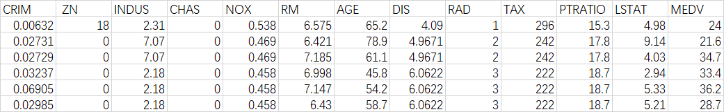
数据库中的每个记录都描述了波士顿的郊区或城镇。数据来自1970年的波士顿标准大都会统计区(SMSA),经过预处理的部分数据如下,其中略去了一个参数
在 Kaggle 上有现成的数据集,数据集直达网址,直接点击 download 就能下载,其数据集跟我使用的数据集具有差距,我将使用我预处理完成的数据集进行多元线性回归问题求解,我将在我的 CSDN 资源上传波斯顿房价数据集的原始数据,Kaggle 数据以及经过我自己预处理的数据,如何在 通过 Kaggle API 下载数据集,参考TensorFlow实现kaggle数据集图像分类Ⅱ——tfrecord数据格式制作,展示,与训练一体综合

波士顿房价数据集解读
波士顿房价数据集包括506个样本,每个样本包括12个特征变量和该地区的平均房价,房价(单价)显然和多个特征变量相关,不是单变量线性回归(一元线性回归)问题,选择多个特征变量来建立线性方程,这就是多变量线性回归(多元线性回归)问题
| 变量 | 含义 |
|---|---|
| CRIM | 城镇人均犯罪率 |
| ZN | 住宅用地超过25,000平方英尺以上的比例 |
| INDUS | 城镇非零售商用土地的比例(即工业或农业等用地比例) |
| CHAS | 查尔斯河虚拟变量(边界是河,则为1;否则为0) |
| NOX | 一氧化氮浓度(百万分之几) |
| RM | 每个住宅的平均房间数 |
| AGE | 1940 年之前建成的自用房屋比例 |
| DIS | 到波士顿五个中心区域的加权距离(与繁华闹市的距离,区分郊区与市区) |
| RAD | 高速公路通行能力指数(辐射性公路的靠近指数) |
| TAX | 每10,000美元的全额财产税率 |
| PTRATIO | 按镇划分的城镇师生比例 |
| B | 1000(Bk-0.63)^2其中Bk是城镇黑人比例 |
| LSTAT | 人口中地位低下者的百分比 |
| MEDV | 自有住房的中位数价值(单位:千美元) |
多元线性回归
多元线性回归原理
房价和多个特征变量相关,波士顿房价采用多元线性回归进行建模,结果可以由不同特征的输入值和对应的权重相乘求和,加上偏置项计算求解
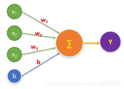
用矩阵表示为
结果由不同特征值的输入值和对应的权重相乘求和,加上偏置项计算求解
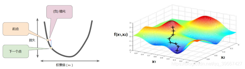
多元线性回归梯度下降
与单变量线性回归不同,多元线性回归的最大问题是容易出现权值越界,多元线性回归具有多个特征值,每一个特征值的取值范围相差各异,最大与最小往往差距几十甚至几百个数量级,在训练时由于不同特征值的权重对神经网络的贡献不同,就容易造成权重的差距也非常大,进而导致权重越界,在训练时出现 NaN 标识,为此需要对每个特征值进行预处理,最常用的预处理方式是归一化,广义的归一化既是将特征值的大小限制在 0~1 之间,常用的归一化方式有除以数据最值,以及设定均值方差标准等
多元线性回归数据预处理
或者
多变量线性回归TensorFLow 1.x 实现
知识储备
numpy 简易矩阵运算
import numpy as np
向量属于矩阵范畴,至少两个维度,如下两个 cell 均为数组
数组
scalar_value = 520
print('scalar_value type:',type(scalar_value))
print('scalar_value:',scalar_value)
try:
    print('scalar_value shape:',scalar_value.shape)
except AttributeError:
    print('INFO:\'int\' object has no attribute \'shape\'')
finally:
    scalar_np = np.array(scalar_value)
    print('INFO:transform scalar to array, we get scalar_np as a array')
print('scalar_np type :', type(scalar_np))
print('scalar_np shape:', scalar_np.shape)
print('scalar_np value:', scalar_np)
scalar_value type: <class 'int'>
scalar_value: 520
INFO:'int' object has no attribute 'shape'
INFO:transform scalar to array, we get scalar_np as a array
scalar_np type : <class 'numpy.ndarray'>
scalar_np shape: ()
scalar_np value: 520
vector_value = [520, 521, 1314]
print('vector_value type:',type(vector_value))
print('vector_value:',vector_value)
try:
    print('scalar_value shape:',vector_value.shape)
except AttributeError:
    print('INFO:\'list\' object has no attribute \'shape\'')
finally:
    vector_np = np.array(vector_value)
    print('INFO:transform list to array, we get vector_np as a array')
print('vector_np type :', type(vector_np))
print('vector_np shape:', vector_np.shape)
print('vector_np value:', vector_np)
vector_value type: <class 'list'>
vector_value: [520, 521, 1314]
INFO:'list' object has no attribute 'shape'
INFO:transform list to array, we get vector_np as a array
vector_np type : <class 'numpy.ndarray'>
vector_np shape: (3,)
vector_np value: [ 520  521 1314]
矩阵
matrix_value = [[520, 521, 1314], [5.20, 5.21, 1.314]]
print('matrix_value type:',type(matrix_value))
print('matrix_value type:',matrix_value)
try:
    print('scalar_value shape:',matrix_value.shape)
except AttributeError:
    print('INFO:\'list\' object has no attribute \'shape\'')
finally:
    matrix_np = np.array(matrix_value)
    print('INFO:transform list to matrix, we get matrix_np as a matrix')
print('matrix_np type :', type(matrix_np))
print('matrix_np shape:', matrix_np.shape)
print('matrix_np value:\n', matrix_np)
matrix_value type: <class 'list'>
matrix_value type: [[520, 521, 1314], [5.2, 5.21, 1.314]]
INFO:'list' object has no attribute 'shape'
INFO:transform list to matrix, we get matrix_np as a matrix
matrix_np type : <class 'numpy.ndarray'>
matrix_np shape: (2, 3)
matrix_np value:
 [[ 520.     521.    1314.   ]
 [   5.2      5.21     1.314]]
行向量
vector_row = np.array([[1, 2, 3]])
print(vector_row, 'shape=', vector_row.shape)
[[1 2 3]] shape= (1, 3)
列向量
vector_column = np.array([[1], [2], [3]])
print(vector_column, 'shape=', vector_column.shape)
[[1]
 [2]
 [3]] shape= (3, 1)
行列转置,使用 numpy.T 进行转置,对任意维度矩阵适用
print(vector_row, 'shape=', vector_row.shape, '\n',
      '*******line*******\n',
      vector_row.T, 'Tshape=', vector_row.T.shape)
[[1 2 3]] shape= (1, 3)
 *******line*******
 [[1]
 [2]
 [3]] Tshape= (3, 1)
matrix = np.array([[1, 2, 3], [4, 5, 6]])
print('raw matrix:\n', matrix,
      '\nraw matrix shape:', matrix.shape,
     '\nTmatrix:\n', matrix.T,
     '\nTmatrix shape:', matrix.T.shape)
raw matrix:
 [[1 2 3]
 [4 5 6]]
raw matrix shape: (2, 3)
Tmatrix:
 [[1 4]
 [2 5]
 [3 6]]
Tmatrix shape: (3, 2)
matrix = np.array([[[1, 2, 3], [4, 5, 6]], [[2, 5, 6], [2, 3, 9]]])
print('raw matrix:\n', matrix,
      '\nraw matrix shape:', matrix.shape,
     '\nTmatrix:\n', matrix.T,
     '\nTmatrix shape:', matrix.T.shape)
raw matrix:
 [[[1 2 3]
  [4 5 6]]

 [[2 5 6]
  [2 3 9]]]
raw matrix shape: (2, 2, 3)
Tmatrix:
 [[[1 2]
  [4 2]]

 [[2 5]
  [5 3]]

 [[3 6]
  [6 9]]]
Tmatrix shape: (3, 2, 2)
矩阵运算仅讨论矩阵乘除,加减太易舍去
点乘有两种方式 ,* & numpy.multiply
matrix_1 = np.array([[1, 2, 3], [4, 5, 6]])
matrix_2 = np.array([[1, 2, 3], [4, 5, 6]])
matrix_result_1 = matrix_1 * matrix_2
matrix_result_2 = np.multiply(matrix_1, matrix_2)
if (matrix_result_1==matrix_result_2).all():
    print('matrix_result_1 is equal to matrix_result_2')
print('matrix_1 multiply matrix_2 is:\n', matrix_result_1)
matrix_result_1 is equal to matrix_result_2
matrix_1 multiply matrix_2 is:
 [[ 1  4  9]
 [16 25 36]]
叉乘只有 matmul 一种计算方式,是线性代数,机器学习,图像处理较为默认的乘法
matrix_1 = np.array([[1, 2, 3], [4, 5, 6]])
matrix_2 = np.array([[1, 2], [3, 4], [5, 6]])
matrix_result_3 = np.matmul(matrix_1, matrix_2)
print('matrix_1 matmul matrix_2 is:\n', matrix_result_3)
matrix_1 matmul matrix_2 is:
 [[22 28]
 [49 64]]
numpy 拓展部分,判断矩阵是否相等
any() 用于每一个元素相对应判断,存在元素相等,则相等
all() 用于判断矩阵是否全等,全部元素相等则相等
判断两个矩阵相等时,最好需要维度相同,维度不同会报严重警告(elementwise comparison failed; this will raise an error in the future),甚至引起程序崩溃
matrix_1 = np.array([[1, 2, 3], [4, 5, 6]])
matrix_2 = np.array([[1, 3, 2], [4, 5, 7]])
矩阵比较返回元素为 bool 值的矩阵
bool_matrix = matrix_1==matrix_2
print('bool_matrix:\n', bool_matrix)
bool_matrix:
 [[ True False False]
 [ True  True False]]
print('matrix_1 is equal to matrix_2 in some positions')
print('bool_matrix.any():', bool_matrix.any())
print('matrix_1 is not equal to matrix_2 in all positions')
print('bool_matrix.all():', bool_matrix.all())
matrix_1 is equal to matrix_2 in some positions
bool_matrix.any(): True
matrix_1 is not equal to matrix_2 in all positions
bool_matrix.all(): False
前请函数解释
pd.read_csv()
官方文档详解函数:pd.read_csv()
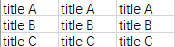
这里主要介绍其中 header 参数,header 表示第几行作为标题,采用的 CSV 示例文件如下
import pandas as pd
for i in range(0, 3):
    demo_frame = pd.read_csv('./data/demo.csv', header=i)
    print('header = %d' % i)
    print(demo_frame)
    if i < 2:
        print('*******----*******')
header = 0
   title A title A.1 title A.2
0  title B   title B   title B
1  title C   title C   title C
*******----*******
header = 1
   title B title B.1 title B.2
0  title C   title C   title C
*******----*******
header = 2
Empty DataFrame
Columns: [title C, title C.1, title C.2]
Index: []
random_normal 函数解析
tensorflow.random_normal(shape, mean=0.0, stddev=1.0, dtype=tf.float32, seed=None, name=None)
从正态分布中输出随机值
参数:
shape: 一维的张量,也是输出的张量
mean: 正态分布的均值
stddev: 正态分布的标准差
dtype: 输出的类型
seed: 一个整数,当设置之后,每次生成的随机数都一样
name: 操作的名字
下面展示了生成一个 N(0, 1)分布的数据
import tensorflow as tf
import matplotlib.pyplot as plt


demo_value=tf.random.normal([1000, 1], mean=0, stddev=1)
with tf.Session() as sess:
    value = sess.run(demo_value)

x_value = []
y_value = []
step = 0.1
neg_boundary = -3
pos_boundary = 3
for i in range(int((pos_boundary - neg_boundary) /step)):
    y =((neg_boundary + i * step < value) & (value < neg_boundary + (i + 1) * step)).sum()
    x_value.append(round((neg_boundary + i * step + step / 2), 3))
    y_value.append(y)

plt.bar(x_value, y_value, width=0.1)
plt.title('Standard normal distribution')
plt.show()

numpy 随机整数生成
numpy.random.randint(low, high=None, size=None, dtype=int)
参数:
low:从分布中得出的最低(带符号)整数(除非 high=None,在这种情况下此参数比最高整数高1)
high:如果设置,则从分布中得出的最大(有符号)整数之上(如果 high=None,则参照上述),如果是数组,则必须包含整数值
size:输出形状。 如果给定的形状是例如(m,n,k),则绘制m * n * k个样本。 默认值为无,在这种情况下,将返回单个值。
dtype:可选,默认值为int。
返回值:
整数的 int 或 ndarray 如果未提供大小,则为单个这样的随机整数
intb = np.random.randint(1, 10)

print('return value:', intb)
return value: 8
导入必要的包
import tensorflow as tf
import matplotlib.pyplot as plt
import numpy as np
import pandas as pd
from sklearn.utils import shuffle
import os
数据读取
等同于 pd.read_csv(‘boston.csv’, header=0)
data_frame = pd.read_csv('./data/boston.csv')
数据描述
data_frame.describe()
| CRIM | ZN | INDUS | CHAS | NOX | RM | AGE | DIS | RAD | TAX | PTRATIO | LSTAT | MEDV | |
|---|---|---|---|---|---|---|---|---|---|---|---|---|---|
| count | 506.000000 | 506.000000 | 506.000000 | 506.000000 | 506.000000 | 506.000000 | 506.000000 | 506.000000 | 506.000000 | 506.000000 | 506.000000 | 506.000000 | 506.000000 |
| mean | 3.613524 | 11.363636 | 11.136779 | 0.069170 | 0.554695 | 6.284634 | 68.574901 | 3.795043 | 9.549407 | 408.237154 | 18.455534 | 12.653063 | 22.532806 |
| std | 8.601545 | 23.322453 | 6.860353 | 0.253994 | 0.115878 | 0.702617 | 28.148861 | 2.105710 | 8.707259 | 168.537116 | 2.164946 | 7.141062 | 9.197104 |
| min | 0.006320 | 0.000000 | 0.460000 | 0.000000 | 0.385000 | 3.561000 | 2.900000 | 1.129600 | 1.000000 | 187.000000 | 12.600000 | 1.730000 | 5.000000 |
| 25% | 0.082045 | 0.000000 | 5.190000 | 0.000000 | 0.449000 | 5.885500 | 45.025000 | 2.100175 | 4.000000 | 279.000000 | 17.400000 | 6.950000 | 17.025000 |
| 50% | 0.256510 | 0.000000 | 9.690000 | 0.000000 | 0.538000 | 6.208500 | 77.500000 | 3.207450 | 5.000000 | 330.000000 | 19.050000 | 11.360000 | 21.200000 |
| 75% | 3.677082 | 12.500000 | 18.100000 | 0.000000 | 0.624000 | 6.623500 | 94.075000 | 5.188425 | 24.000000 | 666.000000 | 20.200000 | 16.955000 | 25.000000 |
| max | 88.976200 | 100.000000 | 27.740000 | 1.000000 | 0.871000 | 8.780000 | 100.000000 | 12.126500 | 24.000000 | 711.000000 | 22.000000 | 37.970000 | 50.000000 |
查看数据值并转为 numpy 格式
使用 pandas 中的 values 与 numpy.array 等价
data_frame.values
array([[6.3200e-03, 1.8000e+01, 2.3100e+00, ..., 1.5300e+01, 4.9800e+00,
        2.4000e+01],
       [2.7310e-02, 0.0000e+00, 7.0700e+00, ..., 1.7800e+01, 9.1400e+00,
        2.1600e+01],
       [2.7290e-02, 0.0000e+00, 7.0700e+00, ..., 1.7800e+01, 4.0300e+00,
        3.4700e+01],
       ...,
       [6.0760e-02, 0.0000e+00, 1.1930e+01, ..., 2.1000e+01, 5.6400e+00,
        2.3900e+01],
       [1.0959e-01, 0.0000e+00, 1.1930e+01, ..., 2.1000e+01, 6.4800e+00,
        2.2000e+01],
       [4.7410e-02, 0.0000e+00, 1.1930e+01, ..., 2.1000e+01, 7.8800e+00,
        1.1900e+01]])
data_frame = np.array(data_frame)
data_frame
array([[6.3200e-03, 1.8000e+01, 2.3100e+00, ..., 1.5300e+01, 4.9800e+00,
        2.4000e+01],
       [2.7310e-02, 0.0000e+00, 7.0700e+00, ..., 1.7800e+01, 9.1400e+00,
        2.1600e+01],
       [2.7290e-02, 0.0000e+00, 7.0700e+00, ..., 1.7800e+01, 4.0300e+00,
        3.4700e+01],
       ...,
       [6.0760e-02, 0.0000e+00, 1.1930e+01, ..., 2.1000e+01, 5.6400e+00,
        2.3900e+01],
       [1.0959e-01, 0.0000e+00, 1.1930e+01, ..., 2.1000e+01, 6.4800e+00,
        2.2000e+01],
       [4.7410e-02, 0.0000e+00, 1.1930e+01, ..., 2.1000e+01, 7.8800e+00,
        1.1900e+01]])
数据归一化,防止训练权值越界
for i in range(data_frame.shape[1] - 1):
    data_frame[:, i] = data_frame[:, i] / (data_frame[:, i].max() - data_frame[:, i].min())
获取数据集
前 11 列作为输入数据 X,最后一列作为预测值 Y
x_data = data_frame[:, :12]
y_data = data_frame[:, 12]
print('x_data:\n', x_data, '\n x_data shape:', x_data.shape,
      '\ny_data:\n', y_data, '\n y_data shape:', y_data.shape)
x_data:
 [[7.10352762e-05 1.80000000e-01 8.46774194e-02 ... 5.64885496e-01
  1.62765957e+00 1.37417219e-01]
 [3.06957815e-04 0.00000000e+00 2.59164223e-01 ... 4.61832061e-01
  1.89361702e+00 2.52207506e-01]
 [3.06733020e-04 0.00000000e+00 2.59164223e-01 ... 4.61832061e-01
  1.89361702e+00 1.11203091e-01]
 ...
 [6.82927750e-04 0.00000000e+00 4.37316716e-01 ... 5.20992366e-01
  2.23404255e+00 1.55629139e-01]
 [1.23176518e-03 0.00000000e+00 4.37316716e-01 ... 5.20992366e-01
  2.23404255e+00 1.78807947e-01]
 [5.32876969e-04 0.00000000e+00 4.37316716e-01 ... 5.20992366e-01
  2.23404255e+00 2.17439294e-01]]
 x_data shape: (506, 12)
y_data:
 [24.  21.6 34.7 33.4 36.2 28.7 22.9 27.1 16.5 18.9 15.  18.9 21.7 20.4
 18.2 19.9 23.1 17.5 20.2 18.2 13.6 19.6 15.2 14.5 15.6 13.9 16.6 14.8
 18.4 21.  12.7 14.5 13.2 13.1 13.5 18.9 20.  21.  24.7 30.8 34.9 26.6
 25.3 24.7 21.2 19.3 20.  16.6 14.4 19.4 19.7 20.5 25.  23.4 18.9 35.4
 24.7 31.6 23.3 19.6 18.7 16.  22.2 25.  33.  23.5 19.4 22.  17.4 20.9
 24.2 21.7 22.8 23.4 24.1 21.4 20.  20.8 21.2 20.3 28.  23.9 24.8 22.9
 23.9 26.6 22.5 22.2 23.6 28.7 22.6 22.  22.9 25.  20.6 28.4 21.4 38.7
 43.8 33.2 27.5 26.5 18.6 19.3 20.1 19.5 19.5 20.4 19.8 19.4 21.7 22.8
 18.8 18.7 18.5 18.3 21.2 19.2 20.4 19.3 22.  20.3 20.5 17.3 18.8 21.4
 15.7 16.2 18.  14.3 19.2 19.6 23.  18.4 15.6 18.1 17.4 17.1 13.3 17.8
 14.  14.4 13.4 15.6 11.8 13.8 15.6 14.6 17.8 15.4 21.5 19.6 15.3 19.4
 17.  15.6 13.1 41.3 24.3 23.3 27.  50.  50.  50.  22.7 25.  50.  23.8
 23.8 22.3 17.4 19.1 23.1 23.6 22.6 29.4 23.2 24.6 29.9 37.2 39.8 36.2
 37.9 32.5 26.4 29.6 50.  32.  29.8 34.9 37.  30.5 36.4 31.1 29.1 50.
 33.3 30.3 34.6 34.9 32.9 24.1 42.3 48.5 50.  22.6 24.4 22.5 24.4 20.
 21.7 19.3 22.4 28.1 23.7 25.  23.3 28.7 21.5 23.  26.7 21.7 27.5 30.1
 44.8 50.  37.6 31.6 46.7 31.5 24.3 31.7 41.7 48.3 29.  24.  25.1 31.5
 23.7 23.3 22.  20.1 22.2 23.7 17.6 18.5 24.3 20.5 24.5 26.2 24.4 24.8
 29.6 42.8 21.9 20.9 44.  50.  36.  30.1 33.8 43.1 48.8 31.  36.5 22.8
 30.7 50.  43.5 20.7 21.1 25.2 24.4 35.2 32.4 32.  33.2 33.1 29.1 35.1
 45.4 35.4 46.  50.  32.2 22.  20.1 23.2 22.3 24.8 28.5 37.3 27.9 23.9
 21.7 28.6 27.1 20.3 22.5 29.  24.8 22.  26.4 33.1 36.1 28.4 33.4 28.2
 22.8 20.3 16.1 22.1 19.4 21.6 23.8 16.2 17.8 19.8 23.1 21.  23.8 23.1
 20.4 18.5 25.  24.6 23.  22.2 19.3 22.6 19.8 17.1 19.4 22.2 20.7 21.1
 19.5 18.5 20.6 19.  18.7 32.7 16.5 23.9 31.2 17.5 17.2 23.1 24.5 26.6
 22.9 24.1 18.6 30.1 18.2 20.6 17.8 21.7 22.7 22.6 25.  19.9 20.8 16.8
 21.9 27.5 21.9 23.1 50.  50.  50.  50.  50.  13.8 13.8 15.  13.9 13.3
 13.1 10.2 10.4 10.9 11.3 12.3  8.8  7.2 10.5  7.4 10.2 11.5 15.1 23.2
  9.7 13.8 12.7 13.1 12.5  8.5  5.   6.3  5.6  7.2 12.1  8.3  8.5  5.
 11.9 27.9 17.2 27.5 15.  17.2 17.9 16.3  7.   7.2  7.5 10.4  8.8  8.4
 16.7 14.2 20.8 13.4 11.7  8.3 10.2 10.9 11.   9.5 14.5 14.1 16.1 14.3
 11.7 13.4  9.6  8.7  8.4 12.8 10.5 17.1 18.4 15.4 10.8 11.8 14.9 12.6
 14.1 13.  13.4 15.2 16.1 17.8 14.9 14.1 12.7 13.5 14.9 20.  16.4 17.7
 19.5 20.2 21.4 19.9 19.  19.1 19.1 20.1 19.9 19.6 23.2 29.8 13.8 13.3
 16.7 12.  14.6 21.4 23.  23.7 25.  21.8 20.6 21.2 19.1 20.6 15.2  7.
  8.1 13.6 20.1 21.8 24.5 23.1 19.7 18.3 21.2 17.5 16.8 22.4 20.6 23.9
 22.  11.9]
 y_data shape: (506,)
定义占位符
x = tf.placeholder(tf.float32, [None, 12], name='X')
y = tf.placeholder(tf.float32, [None, 1], name='Y')
定义命名空间 Model 与 构建模型函数
定义命名空间可以打包节点,让计算图结构更清晰
with tf.name_scope('Model'):
    w = tf.Variable(tf.random_normal([12, 1], stddev=0.01), name='W')
    b = tf.Variable(1.0, name='b')

    def model(x, w, b):
        return tf.matmul(x, w) + b

    pred = model(x, w ,b)
定义损失函数
with tf.name_scope('LossFunction'):
    loss_function = tf.reduce_mean(tf.pow(y - pred, 2))
设置训练参数
epochs = 50
learning_rate = 0.01
定义优化器
optimizer = tf.train.GradientDescentOptimizer(learning_rate).minimize(loss_function)
WARNING:tensorflow:From e:\anaconda3\envs\tensorflow1.x\lib\site-packages\tensorflow_core\python\ops\math_grad.py:1375: where (from tensorflow.python.ops.array_ops) is deprecated and will be removed in a future version.
Instructions for updating:
Use tf.where in 2.0, which has the same broadcast rule as np.where
开始训练
涵盖 Tensorboard
init = tf.global_variables_initializer()

logdir='./boston_logs'

if not os.path.exists(logdir):
    os.mkdir(logdir)

sum_loss_op = tf.summary.scalar('loss', loss_function)
merged = tf.summary.merge_all()

loss_list = []
with tf.Session() as sess:
    writer = tf.summary.FileWriter(logdir, sess.graph)
    sess.run(init)
    for epoch in range(epochs):
        loss_sum = 0
        for xs, ys in zip(x_data, y_data):
            xs = xs.reshape(1, 12)
            ys = ys.reshape(1, 1)

            _, summary_str, loss = sess.run([optimizer, sum_loss_op, loss_function], feed_dict={x:xs, y:ys})
            writer.add_summary(summary_str, epoch)
            loss_sum += loss
        xvalues, yvalues = shuffle(x_data, y_data)
        b0temp = b.eval()
        w0temp = w.eval()
        loss_average = loss_sum / len(y_data)
        loss_list.append(loss_average)
        print('Epoch=%2d/%d' % (epoch + 1, epochs), 'loss=', loss_average, 'b=', b0temp, 'w', w0temp)
部分训练如下
Epoch=45/50 loss= 19.722597667626808 b= 11.380757 w [[ -9.694396  ]
 [  1.7936593 ]
 [ -1.16507   ]
 [  0.08395504]
 [ -1.6580088 ]
 [ 22.879427  ]
 [ -0.75722593]
 [ -7.0394974 ]
 [  5.993214  ]
 [ -5.6059985 ]
 [ -3.022516  ]
 [-20.444736  ]]
Epoch=46/50 loss= 19.706890646352054 b= 11.536841 w [[ -9.75812   ]
 [  1.8009328 ]
 [ -1.1473005 ]
 [  0.08115605]
 [ -1.7400098 ]
 [ 22.876568  ]
 [ -0.76073337]
 [ -7.0966077 ]
 [  6.021573  ]
 [ -5.639438  ]
 [ -3.0393136 ]
 [-20.420984  ]]
Epoch=47/50 loss= 19.691629594227987 b= 11.691801 w [[ -9.819139  ]
 [  1.8077872 ]
 [ -1.1304704 ]
 [  0.07859011]
 [ -1.8202585 ]
 [ 22.87306   ]
 [ -0.76421165]
 [ -7.1523952 ]
 [  6.0486703 ]
 [ -5.6719646 ]
 [ -3.0562222 ]
 [-20.39817   ]]
Epoch=48/50 loss= 19.676788920826354 b= 11.8455925 w [[ -9.877559  ]
 [  1.814242  ]
 [ -1.1145364 ]
 [  0.07624044]
 [ -1.898832  ]
 [ 22.868958  ]
 [ -0.76764995]
 [ -7.206896  ]
 [  6.0745893 ]
 [ -5.7036195 ]
 [ -3.0732188 ]
 [-20.376238  ]]
Epoch=49/50 loss= 19.662351876186804 b= 11.998237 w [[ -9.933487  ]
 [  1.8203168 ]
 [ -1.0994513 ]
 [  0.07409383]
 [ -1.9757991 ]
 [ 22.864248  ]
 [ -0.77103287]
 [ -7.260162  ]
 [  6.09939   ]
 [ -5.7344313 ]
 [ -3.090277  ]
 [-20.355164  ]]
Epoch=50/50 loss= 19.648305257320043 b= 12.149709 w [[ -9.987032  ]
 [  1.8260295 ]
 [ -1.0851728 ]
 [  0.07213799]
 [ -2.0512192 ]
 [ 22.858953  ]
 [ -0.77434844]
 [ -7.312225  ]
 [  6.1231446 ]
 [ -5.764425  ]
 [ -3.1073725 ]
 [-20.33495   ]]
查看计算图

查看损失值
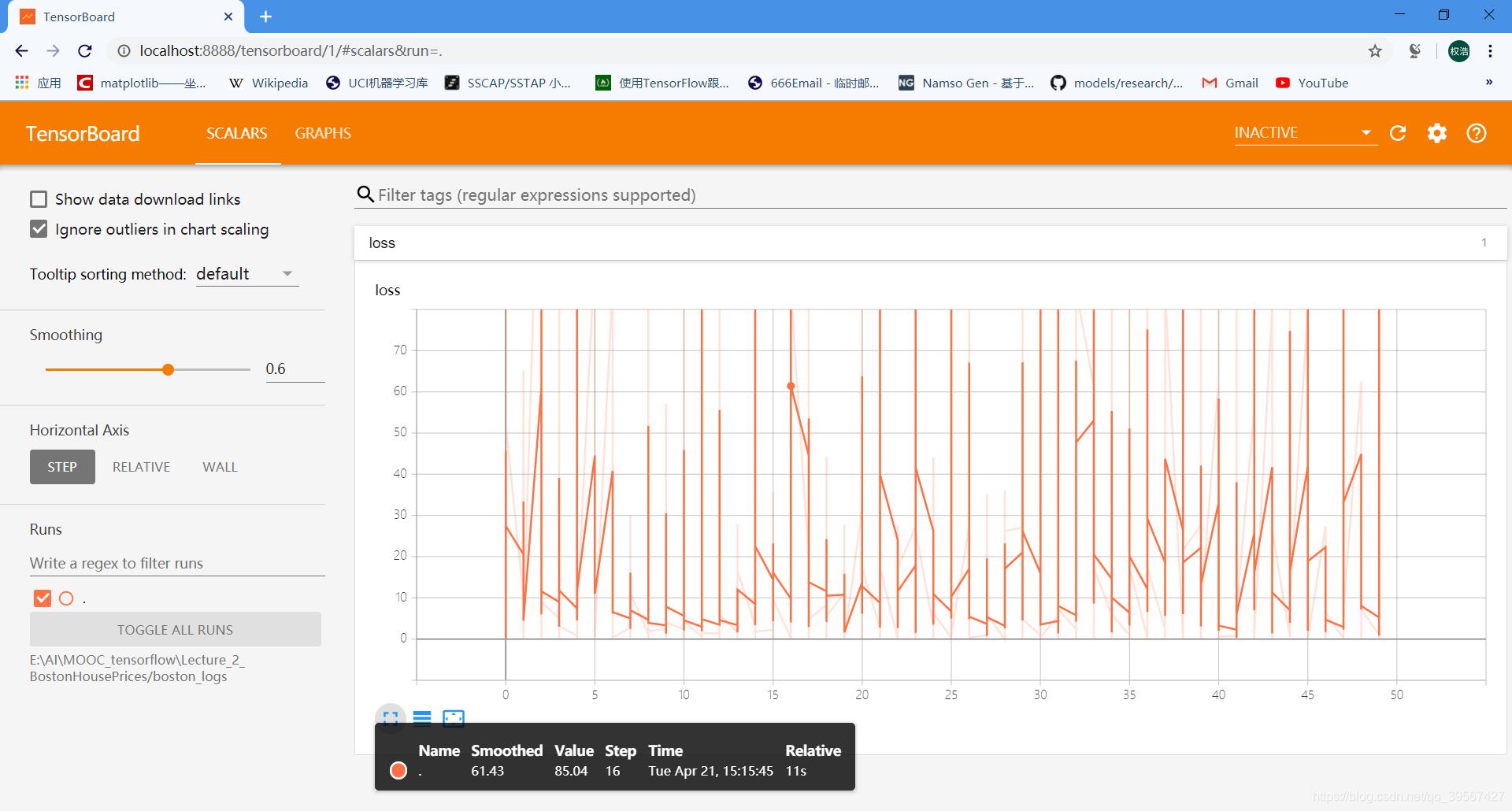
关于如何查看 TensorBoard 参考Tensorflow 笔记 Ⅰ——TensorFlow 编程基础
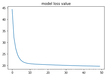
可视化模型损失值
plt.plot(loss_list)
plt.title('model loss value')
plt.show()
模型预测
如果从重新读入的 CSV 文件数据,记得 归一化选出来的值
choose_n = np.random.randint(506)

x_test = x_data[choose_n]
x_test = x_test.reshape(1, 12)

print('The data in boston.csv is the line:', choose_n + 2)
predict = np.matmul(x_test, w0temp) + b0temp
print('Predict value:%f' % predict)

targrt = y_data[choose_n]
print('Target  value:%f' % targrt)
The data in boston.csv is the line: 88
Predict value:17.862059
Target  value:22.500000
多变量线性回归TensorFLow 2.x 实现
前情函数
大部分函数与操作的解释在 Lecture_2_tensorflow1.x.ipynb 中解释过,这里仅解释少量函数
pandas 的 head & detail
head:用于显示前几行数据
tail:用于显示后几行数据
import pandas as pd


demo_frame = pd.read_csv('./data/demo.csv')
demo_frame.head(2)
| title A | title A.1 | title A.2 | |
|---|---|---|---|
| 0 | title B | title B | title B |
| 1 | title C | title C | title C |
demo_frame.head(1)
| title A | title A.1 | title A.2 | |
|---|---|---|---|
| 0 | title B | title B | title B |
demo_frame.tail(1)
| title A | title A.1 | title A.2 | |
|---|---|---|---|
| 1 | title C | title C | title C |
demo_frame.tail(2)
| title A | title A.1 | title A.2 | |
|---|---|---|---|
| 0 | title B | title B | title B |
| 1 | title C | title C | title C |
正式开始
导入必要的包
import tensorflow as tf
import matplotlib.pyplot as plt
import numpy as np
import pandas as pd
from sklearn.utils import shuffle
from sklearn.preprocessing import scale
import os


tf.__version__
'2.0.0'
数据预处理
读取数据并转换为 numpy array 格式
data_frame = pd.read_csv('./data/boston.csv')
data_frame = data_frame.values
data_frame
array([[6.3200e-03, 1.8000e+01, 2.3100e+00, ..., 1.5300e+01, 4.9800e+00,
        2.4000e+01],
       [2.7310e-02, 0.0000e+00, 7.0700e+00, ..., 1.7800e+01, 9.1400e+00,
        2.1600e+01],
       [2.7290e-02, 0.0000e+00, 7.0700e+00, ..., 1.7800e+01, 4.0300e+00,
        3.4700e+01],
       ...,
       [6.0760e-02, 0.0000e+00, 1.1930e+01, ..., 2.1000e+01, 5.6400e+00,
        2.3900e+01],
       [1.0959e-01, 0.0000e+00, 1.1930e+01, ..., 2.1000e+01, 6.4800e+00,
        2.2000e+01],
       [4.7410e-02, 0.0000e+00, 1.1930e+01, ..., 2.1000e+01, 7.8800e+00,
        1.1900e+01]])
获取数据集
x_data = data_frame[:, :12]
y_data = data_frame[:, 12]
print('x_data:\n', x_data, '\n x_data shape:', x_data.shape,
      '\ny_data:\n', y_data, '\n y_data shape:', y_data.shape)
x_data:
 [[6.3200e-03 1.8000e+01 2.3100e+00 ... 2.9600e+02 1.5300e+01 4.9800e+00]
 [2.7310e-02 0.0000e+00 7.0700e+00 ... 2.4200e+02 1.7800e+01 9.1400e+00]
 [2.7290e-02 0.0000e+00 7.0700e+00 ... 2.4200e+02 1.7800e+01 4.0300e+00]
 ...
 [6.0760e-02 0.0000e+00 1.1930e+01 ... 2.7300e+02 2.1000e+01 5.6400e+00]
 [1.0959e-01 0.0000e+00 1.1930e+01 ... 2.7300e+02 2.1000e+01 6.4800e+00]
 [4.7410e-02 0.0000e+00 1.1930e+01 ... 2.7300e+02 2.1000e+01 7.8800e+00]]
 x_data shape: (506, 12)
y_data:
 [24.  21.6 34.7 33.4 36.2 28.7 22.9 27.1 16.5 18.9 15.  18.9 21.7 20.4
 18.2 19.9 23.1 17.5 20.2 18.2 13.6 19.6 15.2 14.5 15.6 13.9 16.6 14.8
 18.4 21.  12.7 14.5 13.2 13.1 13.5 18.9 20.  21.  24.7 30.8 34.9 26.6
 25.3 24.7 21.2 19.3 20.  16.6 14.4 19.4 19.7 20.5 25.  23.4 18.9 35.4
 24.7 31.6 23.3 19.6 18.7 16.  22.2 25.  33.  23.5 19.4 22.  17.4 20.9
 24.2 21.7 22.8 23.4 24.1 21.4 20.  20.8 21.2 20.3 28.  23.9 24.8 22.9
 23.9 26.6 22.5 22.2 23.6 28.7 22.6 22.  22.9 25.  20.6 28.4 21.4 38.7
 43.8 33.2 27.5 26.5 18.6 19.3 20.1 19.5 19.5 20.4 19.8 19.4 21.7 22.8
 18.8 18.7 18.5 18.3 21.2 19.2 20.4 19.3 22.  20.3 20.5 17.3 18.8 21.4
 15.7 16.2 18.  14.3 19.2 19.6 23.  18.4 15.6 18.1 17.4 17.1 13.3 17.8
 14.  14.4 13.4 15.6 11.8 13.8 15.6 14.6 17.8 15.4 21.5 19.6 15.3 19.4
 17.  15.6 13.1 41.3 24.3 23.3 27.  50.  50.  50.  22.7 25.  50.  23.8
 23.8 22.3 17.4 19.1 23.1 23.6 22.6 29.4 23.2 24.6 29.9 37.2 39.8 36.2
 37.9 32.5 26.4 29.6 50.  32.  29.8 34.9 37.  30.5 36.4 31.1 29.1 50.
 33.3 30.3 34.6 34.9 32.9 24.1 42.3 48.5 50.  22.6 24.4 22.5 24.4 20.
 21.7 19.3 22.4 28.1 23.7 25.  23.3 28.7 21.5 23.  26.7 21.7 27.5 30.1
 44.8 50.  37.6 31.6 46.7 31.5 24.3 31.7 41.7 48.3 29.  24.  25.1 31.5
 23.7 23.3 22.  20.1 22.2 23.7 17.6 18.5 24.3 20.5 24.5 26.2 24.4 24.8
 29.6 42.8 21.9 20.9 44.  50.  36.  30.1 33.8 43.1 48.8 31.  36.5 22.8
 30.7 50.  43.5 20.7 21.1 25.2 24.4 35.2 32.4 32.  33.2 33.1 29.1 35.1
 45.4 35.4 46.  50.  32.2 22.  20.1 23.2 22.3 24.8 28.5 37.3 27.9 23.9
 21.7 28.6 27.1 20.3 22.5 29.  24.8 22.  26.4 33.1 36.1 28.4 33.4 28.2
 22.8 20.3 16.1 22.1 19.4 21.6 23.8 16.2 17.8 19.8 23.1 21.  23.8 23.1
 20.4 18.5 25.  24.6 23.  22.2 19.3 22.6 19.8 17.1 19.4 22.2 20.7 21.1
 19.5 18.5 20.6 19.  18.7 32.7 16.5 23.9 31.2 17.5 17.2 23.1 24.5 26.6
 22.9 24.1 18.6 30.1 18.2 20.6 17.8 21.7 22.7 22.6 25.  19.9 20.8 16.8
 21.9 27.5 21.9 23.1 50.  50.  50.  50.  50.  13.8 13.8 15.  13.9 13.3
 13.1 10.2 10.4 10.9 11.3 12.3  8.8  7.2 10.5  7.4 10.2 11.5 15.1 23.2
  9.7 13.8 12.7 13.1 12.5  8.5  5.   6.3  5.6  7.2 12.1  8.3  8.5  5.
 11.9 27.9 17.2 27.5 15.  17.2 17.9 16.3  7.   7.2  7.5 10.4  8.8  8.4
 16.7 14.2 20.8 13.4 11.7  8.3 10.2 10.9 11.   9.5 14.5 14.1 16.1 14.3
 11.7 13.4  9.6  8.7  8.4 12.8 10.5 17.1 18.4 15.4 10.8 11.8 14.9 12.6
 14.1 13.  13.4 15.2 16.1 17.8 14.9 14.1 12.7 13.5 14.9 20.  16.4 17.7
 19.5 20.2 21.4 19.9 19.  19.1 19.1 20.1 19.9 19.6 23.2 29.8 13.8 13.3
 16.7 12.  14.6 21.4 23.  23.7 25.  21.8 20.6 21.2 19.1 20.6 15.2  7.
  8.1 13.6 20.1 21.8 24.5 23.1 19.7 18.3 21.2 17.5 16.8 22.4 20.6 23.9
 22.  11.9]
 y_data shape: (506,)
划分数据集:训练集、验证集、测试集
train_num = 300
valid_num = 100
test_num = len(x_data) - train_num - valid_num

x_train = x_data[:train_num]
y_train = y_data[:train_num]

x_valid = x_data[train_num:train_num + valid_num]
y_valid = y_data[train_num:train_num + valid_num]

x_test = x_data[train_num + valid_num:train_num + valid_num + test_num]
y_test = y_data[train_num + valid_num:train_num + valid_num + test_num]
数据格式转换 tf.float32,便于使用 tensorflow 进行矩阵运算
数据仍然需要归一化,使用 1.x 版本方式归一化如下
for i in range(data_frame.shape[1] - 1): data_frame[:, i] = data_frame[:, i] / (data_frame[:, i].max() - data_frame[:, i].min()) x_train = tf.cast(x_train, dtype=tf.float32) x_valid = tf.cast(x_valid, dtype=tf.float32) x_test = tf.cast(x_test, dtype=tf.float32)
但在 2.x 版本中我们使用 sklearn 的 preprocessing 下的 scale 函数进
行归一化,归一化方式如下,由选取值减去均值再除以方差
代码如下
x_train = tf.cast(scale(x_train), dtype=tf.float32)
x_valid = tf.cast(scale(x_valid), dtype=tf.float32)
x_test = tf.cast(scale(x_test), dtype=tf.float32)
模型构建
定义模型
def model(x, w, b):
    return tf.matmul(x, w) + b
定义损失函数
def loss(x, y, w, b):
    err = model(x, w, b) - y
    squared_err = tf.square(err)
    return tf.reduce_mean(squared_err)
定义梯度计算函数
def grad(x, y, w, b):
    with tf.GradientTape() as tape:
        loss_ = loss(x, y, w, b)
    return tape.gradient(loss_, [w, b])
创建变量
W = tf.Variable(tf.random.normal([12, 1], mean=0.0, stddev=1.0, dtype=tf.float32), name='W')
B = tf.Variable(tf.zeros(1), dtype=tf.float32, name='B')
print(W), print(B)
<tf.Variable 'W:0' shape=(12, 1) dtype=float32, numpy=
array([[ 2.1337633 ],
       [-1.5243678 ],
       [ 1.7605773 ],
       [-0.7097536 ],
       [-0.36367252],
       [-0.33473644],
       [ 0.24133514],
       [ 0.4708158 ],
       [-0.41538587],
       [-1.6086105 ],
       [ 0.9806768 ],
       [-1.5247517 ]], dtype=float32)>
<tf.Variable 'B:0' shape=(1,) dtype=float32, numpy=array([0.], dtype=float32)>


(None, None)
模型训练
设置训练参数
epochs = 50
learning_rate = 0.001
batch_size = 10
定义优化器
optimizer = tf.keras.optimizers.SGD(learning_rate)
开始训练
loss_list_train = []
loss_list_valid = []
total_step = int(train_num / batch_size)

for epoch in range(epochs):
    for step in range(total_step):
        xs = x_train[step * batch_size:(step + 1) * batch_size, :]
        ys = y_train[step * batch_size:(step + 1) * batch_size]

        grads = grad(xs, ys, W, B)
        optimizer.apply_gradients(zip(grads, [W, B]))

    loss_train = loss(x_train, y_train, W, B).numpy()
    loss_valid = loss(x_valid, y_valid, W, B).numpy()
    loss_list_train.append(loss_train)
    loss_list_valid.append(loss_valid)
    print('epoch={:2d}/{:2d}, train_loss={:.4f}, valid_loss={:.4f}'.format(epoch + 1, epochs, loss_train, loss_valid))
epoch= 1/50, train_loss=661.1297, valid_loss=464.9688
epoch= 2/50, train_loss=595.2870, valid_loss=413.7663
epoch= 3/50, train_loss=538.2567, valid_loss=370.4808
epoch= 4/50, train_loss=488.3504, valid_loss=333.3396
epoch= 5/50, train_loss=444.4039, valid_loss=301.1965
epoch= 6/50, train_loss=405.5635, valid_loss=273.2603
epoch= 7/50, train_loss=371.1657, valid_loss=248.9457
epoch= 8/50, train_loss=340.6702, valid_loss=227.7911
epoch= 9/50, train_loss=313.6215, valid_loss=209.4145
epoch=10/50, train_loss=289.6269, valid_loss=193.4886
epoch=11/50, train_loss=268.3423, valid_loss=179.7267
epoch=12/50, train_loss=249.4640, valid_loss=167.8750
epoch=13/50, train_loss=232.7226, valid_loss=157.7073
epoch=14/50, train_loss=217.8788, valid_loss=149.0217
epoch=15/50, train_loss=204.7192, valid_loss=141.6380
epoch=16/50, train_loss=193.0545, valid_loss=135.3952
epoch=17/50, train_loss=182.7158, valid_loss=130.1506
epoch=18/50, train_loss=173.5531, valid_loss=125.7768
epoch=19/50, train_loss=165.4332, valid_loss=122.1613
epoch=20/50, train_loss=158.2376, valid_loss=119.2044
epoch=21/50, train_loss=151.8614, valid_loss=116.8180
epoch=22/50, train_loss=146.2113, valid_loss=114.9246
epoch=23/50, train_loss=141.2046, valid_loss=113.4559
epoch=24/50, train_loss=136.7681, valid_loss=112.3520
epoch=25/50, train_loss=132.8366, valid_loss=111.5602
epoch=26/50, train_loss=129.3527, valid_loss=111.0344
epoch=27/50, train_loss=126.2654, valid_loss=110.7344
epoch=28/50, train_loss=123.5293, valid_loss=110.6251
epoch=29/50, train_loss=121.1045, valid_loss=110.6758
epoch=30/50, train_loss=118.9556, valid_loss=110.8600
epoch=31/50, train_loss=117.0511, valid_loss=111.1544
epoch=32/50, train_loss=115.3631, valid_loss=111.5390
epoch=33/50, train_loss=113.8671, valid_loss=111.9966
epoch=34/50, train_loss=112.5412, valid_loss=112.5122
epoch=35/50, train_loss=111.3661, valid_loss=113.0730
epoch=36/50, train_loss=110.3246, valid_loss=113.6678
epoch=37/50, train_loss=109.4016, valid_loss=114.2875
epoch=38/50, train_loss=108.5836, valid_loss=114.9238
epoch=39/50, train_loss=107.8588, valid_loss=115.5700
epoch=40/50, train_loss=107.2165, valid_loss=116.2204
epoch=41/50, train_loss=106.6475, valid_loss=116.8702
epoch=42/50, train_loss=106.1435, valid_loss=117.5153
epoch=43/50, train_loss=105.6971, valid_loss=118.1525
epoch=44/50, train_loss=105.3019, valid_loss=118.7791
epoch=45/50, train_loss=104.9520, valid_loss=119.3929
epoch=46/50, train_loss=104.6423, valid_loss=119.9921
epoch=47/50, train_loss=104.3685, valid_loss=120.5753
epoch=48/50, train_loss=104.1263, valid_loss=121.1416
epoch=49/50, train_loss=103.9123, valid_loss=121.6903
epoch=50/50, train_loss=103.7233, valid_loss=122.2208
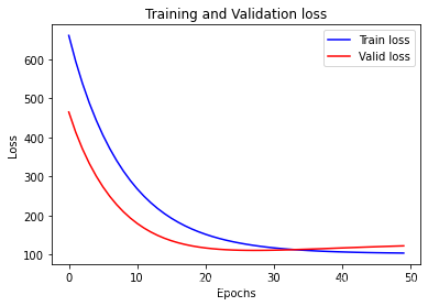
plt.xlabel('Epochs')
plt.ylabel('Loss')
plt.plot(loss_list_train, 'blue', label='Train loss')
plt.plot(loss_list_valid, 'red', label='Valid loss')
plt.legend(loc='best')
plt.title('Training and Validation loss')
plt.show()
查看测试集 loss 值
print('Test_loss:{:.4f}'.format(loss(x_test, y_test, W, B).numpy()))
Test_loss:114.7464
choose_n = np.random.randint(test_num)

y = y_test[choose_n]

print('The data in boston.csv is the line:', choose_n + 402)
predict = model(x_test, W, B)[choose_n]
predict = tf.reshape(predict, ()).numpy()
print('Predict value:%f' % predict)
print('Target  value:%f' % y)
The data in boston.csv is the line: 488
Predict value:25.224939
Target  value:19.100000