数学建模--拟合算法以及Python的三种实现方法

写在前面：
笔记为自行整理，内容出自课程《数学建模学习交流》，主讲人：清风

---

拟合与插值的区别：
插值算法中，得到的多项式 $f(x)$要经过所有样本点。但是如果样本点太多，那
么这个多项式次数过高，会造成龙格现象。
尽管我们可以选择分段的方法避免这种现象，但是更多时候我们更倾向于得到
一个确定的曲线，尽管这条曲线不能经过每一个样本点，但只要保证误差足够小即
可，这就是拟合的思想。 (拟合的结果是得到一个确定的曲线)
拟合曲线的确定：
设样本点为 $(x_i,y_i),i=1,2,...,n$，找到一条曲线 $y=kx+b$，确定 $k,b$的值，使得拟合曲线与样本点最接近。

---

代码实现

import pandas as pd
import numpy as np
import matplotlib.pyplot as plt

np.set_printoptions(suppress=True)  # 不适用科学计数法

x = np.array([8.19,2.72,6.39,8.71,4.7,2.66,3.78])
y = np.array([7.01,2.78,6.47,6.71,4.1,4.23,4.05])

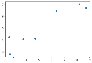
plt.figure()
plt.scatter(x, y)

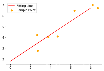
方法一：利用Scipy.leastsq进行拟合

from scipy.optimize import leastsq

# 定义最小二乘函数
def err(p, x, y):
    return p[0] * x + p[1] - y

p0 = [1, 1]  #设置参数初始值，可以随意设置
ret = leastsq(err, p0, args=(x,y))

k,b = ret[0]
print('k=',k)
print('b=',b)

k= 0.6134953486733113
b= 1.7940925476610339

x1 = np.linspace(0,8,100)
y1 = k * x1 + b

plt.scatter(x, y, color="orange",label='Sample Point')
plt.plot(x1,y1,color='red',label='Fitting Line')
plt.legend()

方法二：利用sklearn进行拟合

from sklearn.linear_model import LinearRegression

reg = LinearRegression()

x2 = x.reshape(-1,1)
y2 = y.reshape(-1,1)

reg.fit(x2,y2)

LinearRegression(copy_X=True, fit_intercept=True, n_jobs=None, normalize=False)

reg.intercept_

array([1.79409255])

reg.coef_

array([[0.61349535]])

方法三：利用statsmodels进行拟合

import statsmodels.api as sm

x3 = x
y3 = y
X = sm.add_constant(x3)  # 添加截距项
est = sm.OLS(y3,X)  # 最小二乘法
est2 = est.fit()

est2.summary()

OLS Regression Results

Dep. Variable:	y	R-squared:	0.863
Model:	OLS	Adj. R-squared:	0.835
Method:	Least Squares	F-statistic:	31.46
Date:	Sat, 25 Apr 2020	Prob (F-statistic):	0.00249
Time:	12:50:56	Log-Likelihood:	-5.9456
No. Observations:	7	AIC:	15.89
Df Residuals:	5	BIC:	15.78
Df Model:	1
Covariance Type:	nonrobust

	coef	std err	t	P>|t|	[0.025	0.975]
const	1.7941	0.633	2.833	0.037	0.166	3.422
x1	0.6135	0.109	5.609	0.002	0.332	0.895

Omnibus:	nan	Durbin-Watson:	3.087
Prob(Omnibus):	nan	Jarque-Bera (JB):	0.717
Skew:	0.291	Prob(JB):	0.699
Kurtosis:	1.544	Cond. No.	14.9