如何利用opencv分水岭图像分割算法watershed来分割图像区域?
函数说明:
void watershed( InputArray image, InputOutputArray markers );
image:原图像
markers:包含了轮廓点的数据集合
void distanceTransform(InputArray src, OutputArray dst, int distanceType, int maskSize)
src – 8-bit, 单通道(二值化)输入图片。
dst – 输出结果中包含计算的距离,这是一个32-bit float 单通道的Mat类型数组,大小与输入图片相同。
distanceType – 计算距离的类型那个,可以是 CV_DIST_L1、CV_DIST_L2 、CV_DIST_C。
maskSize – 距离变换掩码矩阵的大小
概述
分水岭算法是一种图像区域分割法,在分割的过程中,它会把跟临近像素间的相似性作为重要的参考依据,从而将在空间位置上相近并且灰度值相近的像素点互相连接起来构成一个封闭的轮廓,封闭性是分水岭算法的一个重要特征。
使用流程
总的概括一下watershed图像自动分割的实现步骤:
- 图像灰度化、滤波、Canny边缘检测
- 查找轮廓,并且把轮廓信息按照不同的编号绘制到watershed的第二个入参merkers上,相当于标记注水点。
- watershed分水岭运算
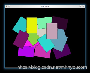
- 绘制分割出来的区域,视觉控还可以使用随机颜色填充,或者跟原始图像融合以下,以得到更好的显示效果。
代码:
JNIEXPORT void JNICALL
Java_org_opencv_samples_tutorial2_Tutorial2Activity_FindFeatures(JNIEnv *, jobject, jlong addrGray,
jlong addrRgba) {
Mat &mGr = *(Mat *) addrGray;
Mat &mRgb = *(Mat *) addrRgba;
vector<KeyPoint> v;
looperAddNum++;
if (looperAddNum > 60) {
looperAddNum = 0;
if (looperIndexNum < 100)
looperIndexNum += 1;
}
// Load the image
Mat src;
cvtColor(mRgb, src, COLOR_RGBA2RGB);
// Check if everything was fine
// Show source image
// Change the background from white to black, since that will help later to extract
// better results during the use of Distance Transform
for( int x = 0; x < src.rows; x++ ) {
for( int y = 0; y < src.cols; y++ ) {
if ( src.at<Vec3b>(x, y) == Vec3b(255,255,255) ) {
src.at<Vec3b>(x, y)[0] = 0;
src.at<Vec3b>(x, y)[1] = 0;
src.at<Vec3b>(x, y)[2] = 0;
}
}
}
// Show output image
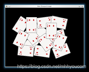
// Create a kernel that we will use for accuting/sharpening our image
Mat kernel = (Mat_<float>(3,3) <<
1, 1, 1,
1, -8, 1,
1, 1, 1); // an approximation of second derivative, a quite strong kernel
// do the laplacian filtering as it is
// well, we need to convert everything in something more deeper then CV_8U
// because the kernel has some negative values,
// and we can expect in general to have a Laplacian image with negative values
// BUT a 8bits unsigned int (the one we are working with) can contain values from 0 to 255
// so the possible negative number will be truncated
Mat imgLaplacian;
Mat sharp = src; // copy source image to another temporary one
filter2D(sharp, imgLaplacian, CV_32F, kernel);//锐化内核
src.convertTo(sharp, CV_32F);
Mat imgResult = sharp - imgLaplacian;
// convert back to 8bits gray scale
imgResult.convertTo(imgResult, CV_8UC3);
imgLaplacian.convertTo(imgLaplacian, CV_8UC3);
// imshow( "Laplace Filtered Image", imgLaplacian );
src = imgResult; // copy back
// Create binary image from source image
Mat bw;
cvtColor(src, bw, CV_BGR2GRAY);
threshold(bw, bw, 40, 255, CV_THRESH_BINARY | CV_THRESH_OTSU);
// Perform the distance transform algorithm
Mat dist;
distanceTransform(bw, dist, CV_DIST_L2, 3);
// Normalize the distance image for range = {0.0, 1.0}
// so we can visualize and threshold it
normalize(dist, dist, 0, 1., NORM_MINMAX);
// Threshold to obtain the peaks
// This will be the markers for the foreground objects
threshold(dist, dist, .4, 1., CV_THRESH_BINARY);
// Dilate a bit the dist image
Mat kernel1 = Mat::ones(3, 3, CV_8UC1);
dilate(dist, dist, kernel1);
// Create the CV_8U version of the distance image
// It is needed for findContours()
Mat dist_8u;
dist.convertTo(dist_8u, CV_8U);
// Find total markers
vector<vector<Point> > contours;
findContours(dist_8u, contours, CV_RETR_EXTERNAL, CV_CHAIN_APPROX_SIMPLE);
// Create the marker image for the watershed algorithm
Mat markers = Mat::zeros(dist.size(), CV_32SC1);
// Draw the foreground markers
for (size_t i = 0; i < contours.size(); i++)
drawContours(markers, contours, static_cast<int>(i), Scalar::all(static_cast<int>(i)+1), -1);
// Draw the background marker
circle(markers, Point(5,5), 3, CV_RGB(255,255,255), -1);
// Perform the watershed algorithm
watershed(src, markers);
// Mat mark = Mat::zeros(markers.size(), CV_8UC1);
// markers.convertTo(mark, CV_8UC1);
// bitwise_not(mark, mark);// 位上取反
// imshow("Markers_v2", mark); // uncomment this if you want to see how the mark
// image looks like at that point
// Generate random colors
vector<Vec3b> colors;
for (size_t i = 0; i < contours.size(); i++)
{
int b = theRNG().uniform(0, 255);
int g = theRNG().uniform(0, 255);
int r = theRNG().uniform(0, 255);
colors.push_back(Vec3b((uchar)b, (uchar)g, (uchar)r));
}
// Create the result image
Mat dst = Mat::zeros(markers.size(), CV_8UC3);
// Fill labeled objects with random colors
for (int i = 0; i < markers.rows; i++)
{
for (int j = 0; j < markers.cols; j++)
{
int index = markers.at<int>(i,j);
if (index > 0 && index <= static_cast<int>(contours.size()))
dst.at<Vec3b>(i,j) = colors[index-1];
else
dst.at<Vec3b>(i,j) = Vec3b(0,0,0);
}
}
cvtColor(dst, mRgb, COLOR_RGB2BGRA);
LOGI("index %d", looperIndexNum);
}
}
效果: