用Python 来做Cluster Analysis

""" 
1. Cluster analysis is a multivariate statistical technique that groups observations on the basis some of their features or variables they are described by. 
2. Observations in a data set can be divided into different groups and sometimes this is very useful. 
3. The final goal of cluster analysis: it is to maximize the similarity of observations within a cluster and maximize the dissimilarity between clusters
4. Classification: Mode (Inputs) -> Outputs -> Correct Values
   Predicting an output category, given input data
5. Clustering: Mode (Inputs) -> Outputs -> ???
   Grouping data points together based on similarities among them and      difference from others.
6. K-means Clustering:
   'K': stands for the number of clusters 
7. 要做K-means clustering 的步骤：
   [1] Choose the number of clusters
   [2] Specify the cluster seeds. (Seed is basically a starting centroid)
   [3] Assign each point to a centroid
   [4] Calculate the centroid
   Repeat the last two steps
"""

import pandas as pd
import numpy as np
import matplotlib.pyplot as plt
import seaborn as sns
sns.set()
from sklearn.cluster import KMeans

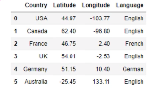
data = pd.read_csv('3.01. Country clusters.csv')  #Load the data
print (data)
print("*******")

代码紧接着上面

# Plot the data
plt.scatter(data['Longitude'], data['Latitude'])
plt.xlim(-180,180)
plt.ylim(-90,90)
plt.show()

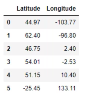
# Select the features
x = data.iloc[:,1:3]
print(x)

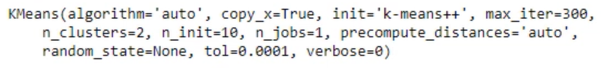
# Clustering
kmeans = KMeans(2)  # The value in brackets in K (the number of clusters)
kmeans.fit(x). #This code will apply k-means clustering with 2 clusters to X

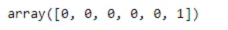
# Clustering results
identified_clusters = kmeans.fit_predict(x)
print(identified_clusters)

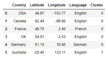
data_with_clusters = data.copy()
data_with_clusters['Cluster'] = identified_clusters
print(data_with_clusters)

plt.scatter(data_with_clusters['Longitude'], data_with_clusters['Latitude'])
plt.xlim(-180,180)
plt.ylim(-90,90)
plt.show()

plt.scatter(data_with_clusters['Longitude'], data_with_clusters['Latitude'], c=data_with_clusters['Cluster'], cmap='rainbow')
plt.xlim(-180,180)
plt.ylim(-90,90)
plt.show()

# Map the data
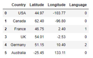
data_mapped = data.copy()
data_mapped['Language'] = data_mapped['Language'].map({'English':0, 'French':1, 'German':2})
print(data_mapped)

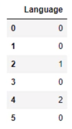
# Select the features
x = data_mapped.iloc[:,3:4]

# Clustering
kmeans = KMeans(3)  # The value in brackets in K (the number of clusters)
kmeans.fit(x). #This code will apply k-means clustering with 2 clusters to X

# Clustering results
identified_clusters = kmeans.fit_predict(x)
print(identified_clusters)

data_with_clusters = data.copy()
data_with_clusters['Cluster'] = identified_clusters
print(data_with_clusters)

plt.scatter(data_with_clusters['Longitude'], data_with_clusters['Latitude'])
plt.xlim(-180,180)
plt.ylim(-90,90)
plt.show()

plt.scatter(data_with_clusters['Longitude'], data_with_clusters['Latitude'], c=data_with_clusters['Cluster'], cmap='rainbow')
plt.xlim(-180,180)
plt.ylim(-90,90)
plt.show()

1. Distance between points in a cluster, "Within-cluster sum of squares’, or WCSS
2. WCSS similar to sst, ssr and sse, WCSS is a measure developed within the ANOVA framework. If we minimize WCSS, we have reached the perfect clustering solution.

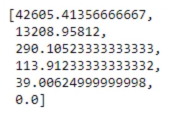
# WCSS
kmeans.inertia_

wcss = []
for i in range(1,7):
  kmeans = KMeans(i)
  kmeans.fit(x)
  wcss_iter = kmeans.inertia_
  wcss.append(wcss_iter)

print(wcss)

# The Elbow Method
number_clusters = range(1,7)
plt.plot(number_clusters,wcss)
plt.title('The Elbow Method')
plt.xlabel('Number of clusters')
plt.ylabel('Within-cluster Sum of Squares')
plt.show() # A two cluster solution would be suboptimal as the leap from 2 to 3 is very big

Pros and Cons of K-Means Clustering:
Pros: 1. Simple to understand
2. Fast to cluster
3. Widely available
4. Easy to implement
5. Always yields a result (Also a con, as it may be deceiving)

Cons	Remedies
1. We need to pick K	1. The Elbow method
2. Sensitive to initialization	2. k-means++
3. Sensitive to outliers	3. Remove outliers
4. Produces spherical soulution
5. Standardization