# import the relevant librariesimport numpy as np # mathematical operationimport matplotlib.pyplot as plt # nice graphsfrom mpl_toolkits.mplot3d import Axes3D # Nice 3D graphs# Generate random input data to train on
observations =1000
xs = np.random.uniform(low=-10, high=10, size=(observations,1))
zs = np.random.uniform(-10,10,(observations,1))
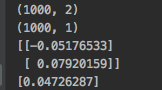
inputs = np.column_stack((xs,zs))print(inputs.shape)# Create the targets we will aim at
noise = np.random.uniform(-1,1,(observations,1))
targets =2*xs -3*zs +5+ noise
print(targets.shape)# Plot the training data"""
In order to use the 3D plot, the objects should have a certain shape, so we reshape the targets.
The proper method to use is reshape and takes as arguments the dimensions in which we want to fit the object.
"""
targets = targets.reshape(observations,)# Plotting according to the conventional matplotlib.pyplot syntax# Declare the figure
fig = plt.figure()# A method allowing us to create the 3D plot
ax = fig.add_subplot(111, projection='3d')# Choose the axes
ax.plot(xs,zs,targets)# Set Labels
ax.set_xlabel('xs')
ax.set_ylabel('zs')
ax.set_zlabel('Targets')# You can fiddle with the azim parameter to plot the data from different angles. Just change the value of azim = 100# to azim = 0; azim = 200, or whatever. Check and see what happens
ax.view_init(azim=100)# So far we were just describing the plot. This method actually shows the plot.
plt.show()
targets = targets.reshape(observations,1)# Initialize variables
init_range =0.1
weights = np.random.uniform(-init_range, init_range, size=(2,1))
biases = np.random.uniform(-init_range, init_range, size=1)# In machine learning, there are many biases as there are outputsprint(weights)print(biases)# Setting a learning rate
learning_rate =0.02# Train the modelfor i inrange(100):
outputs = np.dot(inputs, weights)+ biases # inputs = 1000*2, weights = 2*1 outputs = 1000*1 biases = scalar
deltas = outputs - targets # deltas = 1000*1 outputs = 1000*1 targets = 1000*1
loss = np.sum(deltas **2)/2/observations
print(loss)
deltas_scaled = deltas/observations
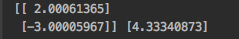
weights = weights - learning_rate * np.dot(inputs.T, deltas_scaled)# weights = 2*1, learning_rate = scalar, inputs.T = 2*1000, deltas_scaled=1000*1
biases = biases - learning_rate * np.sum(deltas_scaled)print(weights, biases)# plot last outputs vs targets
plt.plot(outputs, targets)
plt.xlabel('outputs')
plt.ylabel('targets')
plt.show()