[Hands On ML] 3. 分类（MNIST手写数字预测）

文章目录

1. 数据预览
2. 数据集拆分
3. 二分类
4. 性能评估

4.1 交叉验证
4.2 准确率、召回率
4.3 受试者工作特征（ROC）曲线

5. 多分类
6. 误差分析

6.1 检查混淆矩阵

本文为《机器学习实战：基于Scikit-Learn和TensorFlow》的读书笔记。
中文翻译参考

数据集为70000张手写数字图片，MNIST 数据集下载

1. 数据预览

导入数据

from scipy.io import loadmat
data = loadmat('mnist-original.mat')
data

{'__header__': b'MATLAB 5.0 MAT-file Platform: posix, Created on: Sun Mar 30 03:19:02 2014',
 '__version__': '1.0',
 '__globals__': [],
 'mldata_descr_ordering': array([[array(['label'], dtype='<U5'), array(['data'], dtype='<U4')]],
       dtype=object),
 'data': array([[0, 0, 0, ..., 0, 0, 0],
        [0, 0, 0, ..., 0, 0, 0],
        [0, 0, 0, ..., 0, 0, 0],
        ...,
        [0, 0, 0, ..., 0, 0, 0],
        [0, 0, 0, ..., 0, 0, 0],
        [0, 0, 0, ..., 0, 0, 0]], dtype=uint8),
 'label': array([[0., 0., 0., ..., 9., 9., 9.]])}

数据是一个字典，它的 keys

data.keys()

dict_keys(['__header__', '__version__', '__globals__', 'mldata_descr_ordering', 'data', 'label'])

label 标签是啥，数字图片的数是多少

y = data['label'].ravel()
# y.shape
y

array([0., 0., 0., ..., 9., 9., 9.])

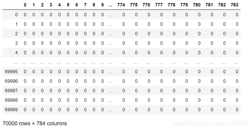
数据是啥，70000行，784列（28*28的图片）

data['data']

array([[0, 0, 0, ..., 0, 0, 0],
       [0, 0, 0, ..., 0, 0, 0],
       [0, 0, 0, ..., 0, 0, 0],
       ...,
       [0, 0, 0, ..., 0, 0, 0],
       [0, 0, 0, ..., 0, 0, 0],
       [0, 0, 0, ..., 0, 0, 0]], dtype=uint8)

import pandas as pd
X = pd.DataFrame(data['data'].T)
X
# print(X.shape)

在这里插入图片描述

选一个数据看看

%matplotlib inline
import numpy as np
import matplotlib
import matplotlib.pyplot as plt
some_digit = np.array(X.iloc[36000,])
some_digit_img = some_digit.reshape(28,28)
plt.imshow(some_digit_img, interpolation='nearest')
# plt.axis('off')
plt.show()

在这里插入图片描述
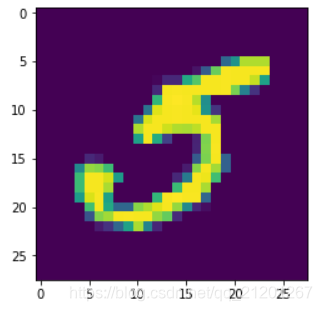
看起来像是5，y[36000]，输出5.0，确实是5

2. 数据集拆分

MNIST 数据集已经事先被分成了一个训练集（前 60000 张图片）和一个测试集（最后 10000 张图片）

X_train, x_test, y_train, y_test = X[:60000], X[60000:], y[:60000], y[60000:]

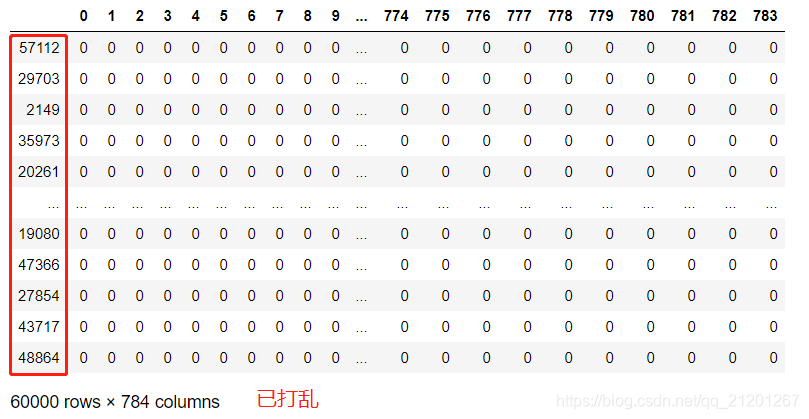
数据集是顺序的（1-9），我们打乱数据：

避免交叉验证的某一折里，没有某个数字
有些算法对训练样本的顺序是敏感的，避免

import numpy as np
shuffle_idx = np.random.permutation(60000)
X_train, y_train = X_train.iloc[shuffle_idx], y_train[shuffle_idx]
X_train

在这里插入图片描述

3. 二分类

选择随机梯度下降模型、训练一个二分类器，预测是不是数字5

y_train_5 = (y_train == 5)
y_test_5 = (y_test == 5)
from sklearn.linear_model import SGDClassifier
sgd_clf = SGDClassifier(random_state=1)
sgd_clf.fit(X_train, y_train_5)

sgd_clf.predict([some_digit])
array([ True]) # 预测上面那张图片是5，答对了

4. 性能评估

4.1 交叉验证

手写版

from sklearn.model_selection import StratifiedKFold
from sklearn.base import clone

# 分层采样（前一章介绍过），分成3份
skfolds = StratifiedKFold(n_splits=3)
for train_index, test_index in skfolds.split(X_train, y_train_5):
    # 采用上面的模型的clone版本
    clone_clf = clone(sgd_clf)
    
    X_train_folds = X_train.iloc[train_index]
    y_train_folds = (y_train_5[train_index])
    X_test_fold = X_train.iloc[test_index]
    y_test_fold = (y_train_5[test_index])
    
    clone_clf.fit(X_train_folds, y_train_folds)
    y_pred = clone_clf.predict(X_test_fold)
    
    n_correct = sum(y_pred == y_test_fold)
    print(n_correct / len(y_pred))

0.9464
0.9472
0.9659

sklearn 内置版

from sklearn.model_selection import cross_val_score
cross_val_score(sgd_clf, X_train, y_train_5, cv=3, scoring='accuracy')
# array([0.9464, 0.9472, 0.9659])

写一个预测不是5的分类器，直接返回全部不是5

from sklearn.base import BaseEstimator
class not5(BaseEstimator):
    def fit(self,X,y=None):
        pass
    def predict(self,X):
        return np.zeros((len(X),1),dtype=bool) # 返回全部不是5
not5_clf = not5()
cross_val_score(not5_clf,X_train,y_train_5,cv=3,scoring='accuracy')
# array([0.91015, 0.90745, 0.91135])

因为只有 10% 的图片是数字 5，总是猜测某张图片不是 5，也有90%的可能性是对的。

这证明了为什么精度通常来说不是一个好的性能度量指标，特别是当你处理有偏差的数据集，比方说其中一些类比其他类频繁得多

4.2 准确率、召回率

精度不是一个好的性能指标
混淆矩阵（准确率、召回率）

# 混淆矩阵
from sklearn.model_selection import cross_val_predict
y_train_pred = cross_val_predict(sgd_clf, X_train, y_train_5, cv=3)

from sklearn.metrics import confusion_matrix
confusion_matrix(y_train_5, y_train_pred)

# output
array([[52625,  1954],
       [  856,  4565]], dtype=int64)

在这里插入图片描述

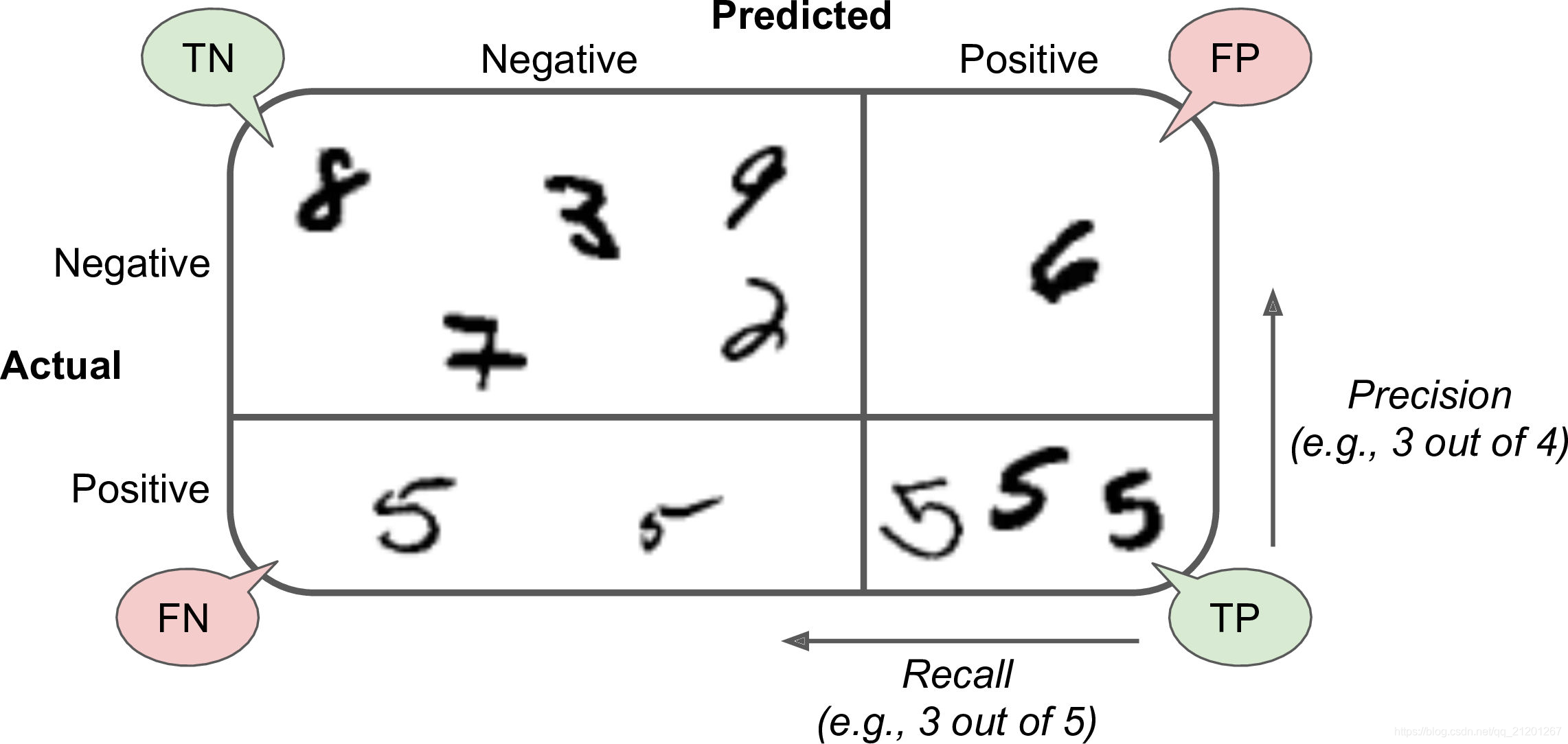
准确率、召回率、F1值(前两者的平均)

$F 1=\frac{2}{\frac{1}{\text {precision}}+\frac{1}{\text {recall}}}=2 * \frac{\text {precison } * \text {recall}}{\text {precison }+\text {recall}}=\frac{T P}{T P+\frac{F N+F P}{2}}$

from sklearn.metrics import precision_score, recall_score
precision_score(y_train_5, y_train_pred) # 0.7002607761926676
recall_score(y_train_5, y_train_pred) # 0.8420955543257701

from sklearn.metrics import f1_score
f1_score(y_train_5, y_train_pred) # 0.7646566164154103

选择标准，看需求而定：

儿童阅读，希望过滤不适合的，我们希望高的准确率，标记成适合的，里面真的适合的比例要很高，极大限度保护儿童
视频警报预测，则希望高的召回率，是危险的，不能报不危险
F1值则要求两者都要比较高

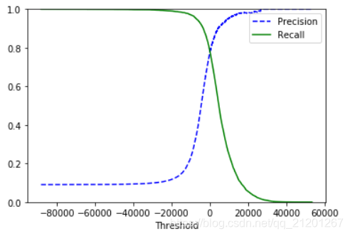
准确率与召回率的折衷：

提高决策阈值，可以提高准确率，降低召回率
降低决策阈值，可以提高召回率，降低准确率

在这里插入图片描述

y_scores = cross_val_predict(sgd_clf,X_train,y_train_5,cv=3,
                            method='decision_function')
from sklearn.metrics import precision_recall_curve
# help(precision_recall_curve)
precisions, recalls, thresholds = precision_recall_curve(y_train_5, y_scores)

def plot_precision_recall_vs_threshold(precisions, recalls, thresholds):
    plt.plot(thresholds, precisions[:-1], "b--", label="Precision")
    plt.plot(thresholds, recalls[:-1], "g-", label="Recall")
    plt.xlabel("Threshold")
    plt.legend(loc="best")
    plt.ylim([0, 1])
plot_precision_recall_vs_threshold(precisions, recalls, thresholds)
plt.show()

在这里插入图片描述
直接画出准确率与召回率的关系

def plot_precision_recall(precisions, recalls):
    plt.plot(recalls[:-1], precisions[:-1], "b--", label="Recalls VS Precisions")
    plt.xlabel("Recalls")
    plt.ylabel("Precisions")
    plt.legend(loc="best")
    plt.ylim([0, 1])
plot_precision_recall(precisions, recalls)
plt.show()

在这里插入图片描述

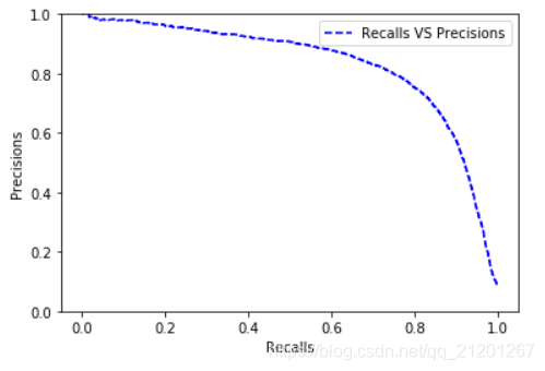
找到准确率 90%的点，其召回率为 52%

threshold_90_precision = thresholds[np.argmax(precisions >= 0.9)]
y_train_pred_90 = (y_scores >= threshold_90_precision)
precision_score(y_train_5, y_train_pred_90) # 0.9000318369945877
recall_score(y_train_5, y_train_pred_90)  # 0.5214904999077661

4.3 受试者工作特征（ROC）曲线

ROC 曲线是真正例率（true positive rate，召回率）对假正例率（false positive rate, FPR 反例被错误分成正例的比率）的曲线

from sklearn.metrics import roc_curve
# help(roc_curve)
fpr, tpr, thresholds = roc_curve(y_train_5, y_scores)

def plot_roc_curve(fpr, tpr, label=None):
    plt.plot(fpr, tpr, linewidth=2, label=label)
    plt.plot([0, 1], [0, 1], 'k--')
    plt.axis([0, 1, 0, 1])
    plt.xlabel('False Positive Rate')
    plt.ylabel('True Positive Rate')
plot_roc_curve(fpr, tpr)
plt.show()

在这里插入图片描述
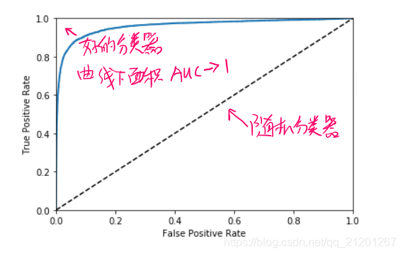
比较分类器优劣的方法是：测量ROC曲线下的面积（AUC），面积越接近1越好

完美的分类器的 ROC AUC 等于 1
纯随机分类器的 ROC AUC 等于 0.5

from sklearn.metrics import roc_auc_score
roc_auc_score(y_train_5, y_scores) # 0.9603458830084456

随机森林模型对比

from sklearn.ensemble import RandomForestClassifier
forest_clf = RandomForestClassifier(random_state=42)
y_probas_forest = cross_val_predict(forest_clf, X_train, y_train_5, cv=3,
                                    method="predict_proba")
help(RandomForestClassifier.predict_proba)
#  Returns
#     -------
#     p : array of shape (n_samples, n_classes), or a list of n_outputs
#         such arrays if n_outputs > 1.
#         The class probabilities of the input samples. The order of the
#         classes corresponds to that in the attribute :term:`classes_`.

y_scores_forest = y_probas_forest[:, 1] # score = proba of positive class
fpr_forest, tpr_forest, thresholds_forest = roc_curve(y_train_5,y_scores_forest)
plt.plot(fpr, tpr, "b:", label="SGD")
plot_roc_curve(fpr_forest, tpr_forest, "Random Forest")
plt.legend(loc="best")
plt.show()

在这里插入图片描述

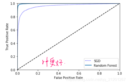
roc_auc_score(y_train_5, y_scores_forest) # 0.9982577037448723

5. 多分类

一些算法（比如，随机森林，朴素贝叶斯）可以直接处理多类分类问题
其他一些算法（比如 SVM 或线性分类器）则是严格的二分类器

但是：可以可以把二分类用于多分类当中

上面的数字预测：

一个方法是：训练10个二分类器（是n吗？不是n吗？n=0-9）。一个样本进行10次分类，选出决策分数最高。这叫做“一对所有”（OvA）策略（也被叫做“一对其他”，OneVsRest）
另一个策略是对每2个数字都训练一个二分类器：一个分类器用来处理数字 0 和数字 1，一个用来处理数字 0 和数字 2，一个用来处理数字 1 和 2，以此类推。
这叫做“一对一”（OvO）策略。如果有 N 个类。你需要训练N*(N-1)/2个分类器。选出胜出的分类器

OvO主要优点是：每个分类器只需要在训练集的部分数据上面进行训练。这部分数据是它所需要区分的那两个类对应的数据

对于大部分的二分类器来说，OvA 是更好的选择

sgd_clf.fit(X_train, y_train)
sgd_clf.predict([some_digit])  # array([5.])

随机梯度下降分类器探测到是多分类，训练了10个分类器，分别作出决策

some_digit_scores = sgd_clf.decision_function([some_digit])
some_digit_scores

array([[ -3868.24582957, -27686.91834291, -11576.99227803,
         -1167.01579458, -21161.58664081,   1445.95448704,
        -20347.02376541, -11273.60667573, -19012.16864028,
        -12849.63656789]])

np.argmax(some_digit_scores) # 5
sgd_clf.classes_ # array([0., 1., 2., 3., 4., 5., 6., 7., 8., 9.])
sgd_clf.classes_[5] # 5.0

label 5 获得的决策值最大，所以预测为 5

强制 Scikit-Learn 使用 OvO 策略或者 OvA 策略
你可以使用OneVsOneClassifier类或者OneVsRestClassifier类。传递一个二分类器给它的构造函数

from sklearn.multiclass import OneVsOneClassifier
ovo_clf = OneVsOneClassifier(SGDClassifier(random_state=1))
ovo_clf.fit(X_train, y_train)
ovo_clf.predict([some_digit]) # array([5.])

len(ovo_clf.estimators_) # 45，组合数 C-n-2

对于随机森林模型，不必使用上面的策略，它可以进行多分类

forest_clf.fit(X_train, y_train)
forest_clf.predict([some_digit]) # array([5.])
forest_clf.predict_proba([some_digit])
# array([[0.04, 0.  , 0.02, 0.05, 0.  , 0.88, 0.  , 0.  , 0.01, 0.  ]])
# label 5 的概率最大

6. 误差分析

6.1 检查混淆矩阵

使用cross_val_predict()做出预测，然后调用confusion_matrix()函数

y_train_pred = cross_val_predict(sgd_clf, X_train, y_train, cv=3)
conf_mat = confusion_matrix(y_train, y_train_pred)
conf_mat

array([[5777,    0,   24,   21,   10,   19,   22,    4,   36,   10],
       [   3, 6478,   48,   46,   12,   25,   12,   14,   83,   21],
       [  91,   71, 5088,  235,   38,   40,   77,   64,  235,   19],
       [  56,   26,  185, 5376,    6,  160,   32,   62,  143,   85],
       [  41,   34,   69,   49, 5055,   36,   64,   40,  174,  280],
       [  95,   27,   66,  430,   65, 4243,   98,   23,  275,   99],
       [ 101,   20,   82,   14,   31,   98, 5501,    3,   58,   10],
       [  38,   27,   88,   79,   47,   21,    5, 5650,   33,  277],
       [  61,  130,   96,  469,   31,  240,   40,   39, 4587,  158],
       [  51,   34,   50,  250,  141,   80,    1,  330,  289, 4723]],
      dtype=int64)

用图像展现混淆矩阵

plt.matshow(conf_mat, cmap=plt.cm.gray)

在这里插入图片描述
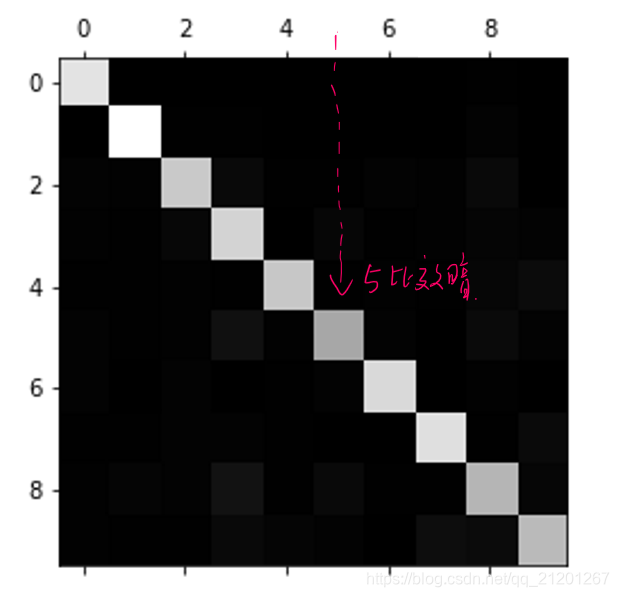
白色主要在对角线上，意味着被分类正确。
数字 5 对应的格子比其他的要暗。两种可能：数据5比较少，数据5预测不准确

row_sums = conf_mat.sum(axis=1, keepdims=True)
norm_conf_mat = conf_mat/row_sums # 转成概率
np.fill_diagonal(norm_conf_mat, 0) # 对角线的抹去
plt.matshow(norm_conf_mat, cmap=plt.cm.gray)
plt.show()

只保留被错误分类的数据，再查看错误分布：

在这里插入图片描述
可以看出，数字被错误的预测成3、8、9的较多

把3和5的预测情况拿出来分析
def plot_digits(instances, images_per_row=10, **options):
    size = 28
    images_per_row = min(len(instances), images_per_row)
    images = [instance.reshape(size,size) for instance in instances]
    n_rows = (len(instances) - 1) // images_per_row + 1
    row_images = []
    n_empty = n_rows * images_per_row - len(instances)
    images.append(np.zeros((size, size * n_empty)))
    for row in range(n_rows):
        rimages = images[row * images_per_row : (row + 1) * images_per_row]
        row_images.append(np.concatenate(rimages, axis=1))
    image = np.concatenate(row_images, axis=0)
    plt.imshow(image, cmap = plt.cm.binary, **options)
    plt.axis("off")

cl_a, cl_b = 3, 5
X_aa = X_train[(y_train == cl_a) & (y_train_pred == cl_a)]
X_ab = X_train[(y_train == cl_a) & (y_train_pred == cl_b)]
X_ba = X_train[(y_train == cl_b) & (y_train_pred == cl_a)]
X_bb = X_train[(y_train == cl_b) & (y_train_pred == cl_b)]
plt.figure(figsize=(8,8))
plt.subplot(221); plot_digits(np.array(X_aa[:25]), images_per_row=5)
plt.subplot(222); plot_digits(np.array(X_ab[:25]), images_per_row=5)
plt.subplot(223); plot_digits(np.array(X_ba[:25]), images_per_row=5)
plt.subplot(224); plot_digits(np.array(X_bb[:25]), images_per_row=5)
plt.show()

原因：3 和 5 的不同像素很少，所以模型容易混淆
在这里插入图片描述

3 和 5 之间的主要差异是连接顶部的线和底部的线的细线的位置。
如果你画一个 3，连接处稍微向左偏移，分类器很可能将它分类成5。反之亦然。换一个说法，这个分类器对于图片的位移和旋转相当敏感。
所以，减轻 3、5 混淆的一个方法是对图片进行预处理，确保它们都很好地中心化和不过度旋转。这同样很可能帮助减轻其他类型的错误。