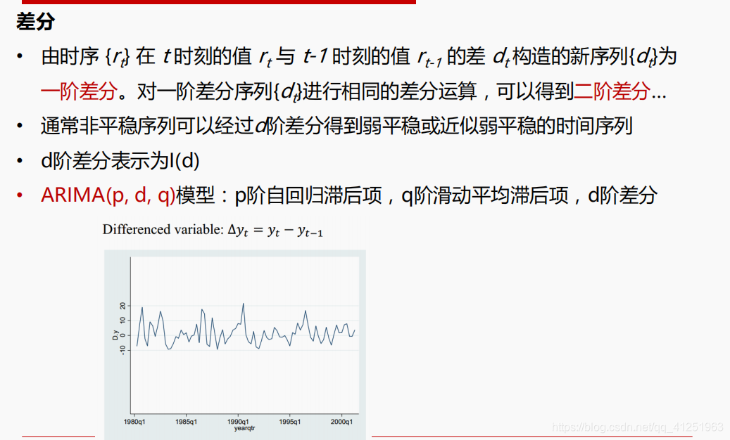
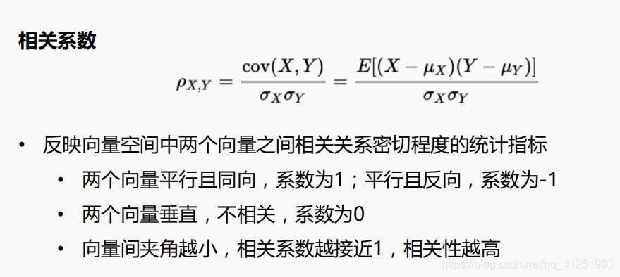
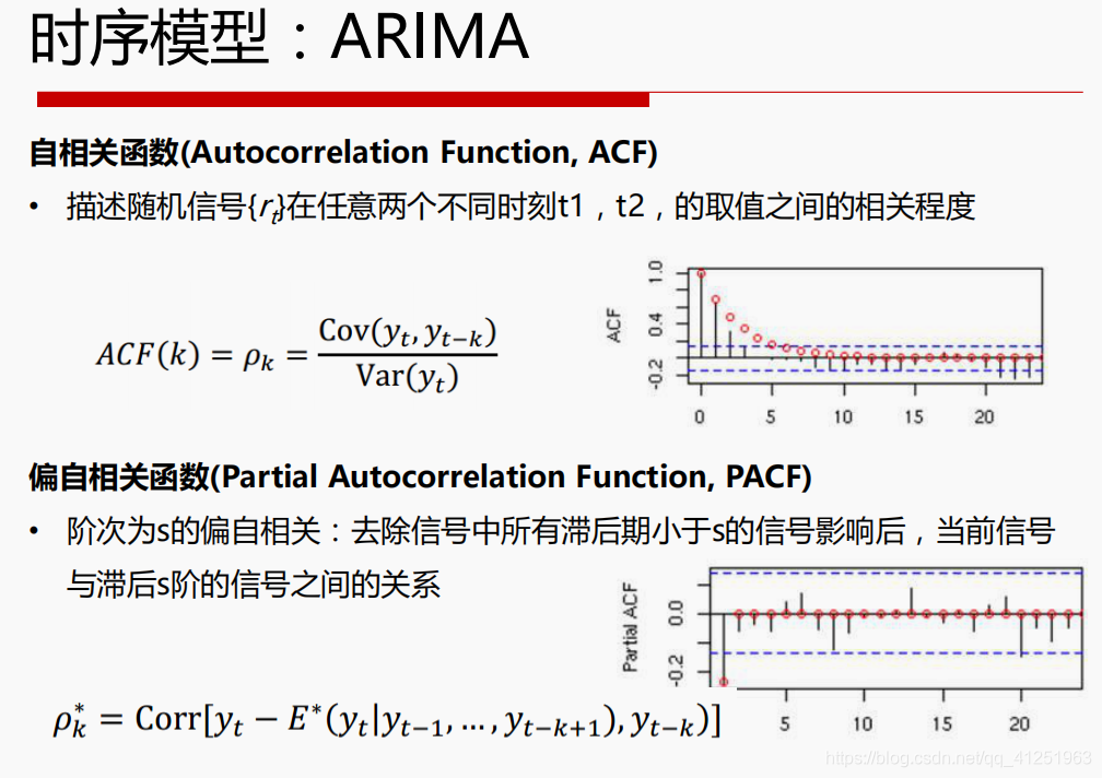
Python的日期和时间处理及操作
python中日期和时间格式化输出的方法
https://blog.csdn.net/qq_41251963/article/details/81874047
Python的日期和时间处理
datetime模块
from datetime import datetime
now = datetime.now()
print(now)
2020-02-06 10:10:53.182169
print('年: {}, 月: {}, 日: {}'.format(now.year, now.month, now.day))
年: 2020, 月: 2, 日: 6
diff = datetime(2020, 3, 4, 17) - datetime(1998, 2, 18, 15)
print(type(diff))
print(diff)
print('经历了{}天, {}秒。'.format(diff.days, diff.seconds))
<class 'datetime.timedelta'>
8050 days, 2:00:00
经历了8050天, 7200秒。
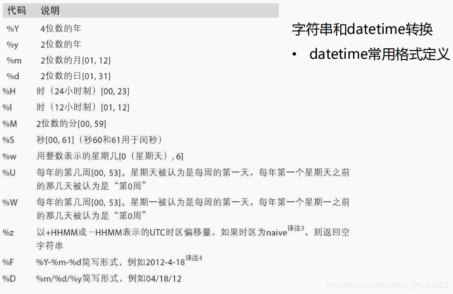
字符串和datetime转换
datetime -> str
# str()
dt_obj = datetime(2020, 2, 2)
str_obj = str(dt_obj)
print(type(str_obj))
print(str_obj)
<class 'str'>
2020-02-02 00:00:00
# datetime.strftime()
str_obj2 = dt_obj.strftime('%d-%m-%Y')
print(str_obj2)
02-02-2020
str -> datetime
# strptime
dt_str = '2020-02-02'
dt_obj2 = datetime.strptime(dt_str, '%Y-%m-%d')
print(type(dt_obj2))
print(dt_obj2)
<class 'datetime.datetime'>
2020-02-02 00:00:00
# dateutil.parser.parse
from dateutil.parser import parse
dt_str2 = '2020/02/02'
dt_obj3 = parse(dt_str2)
print(type(dt_obj3))
print(dt_obj3)
<class 'datetime.datetime'>
2020-02-02 00:00:00
# pd.to_datetime
import pandas as pd
s_obj = pd.Series(['2020/02/01', '2020/02/02', '2020-02-02', '2020-02-02'], name='course_time')
print(s_obj)
0    2020/02/01
1    2020/02/02
2    2020-02-02
3    2020-02-02
Name: course_time, dtype: object
s_obj2 = pd.to_datetime(s_obj)
print(s_obj2)
0   2020-02-01
1   2020-02-02
2   2020-02-02
3   2020-02-02
Name: course_time, dtype: datetime64[ns]
# 处理缺失值
s_obj3 = pd.Series(['2020/02/01', '2020/02/02', '2020-02-03', '2020-02-04'] + [None],
                   name='course_time')
print(s_obj3)
0    2020/02/01
1    2020/02/02
2    2020-02-03
3    2020-02-04
4          None
Name: course_time, dtype: object
s_obj4 = pd.to_datetime(s_obj3)
print(s_obj4) # NAT-> Not a Time
Pandas的时间序列处理
创建
from datetime import datetime
import pandas as pd
import numpy as np

# 指定index为datetime的list
date_list = [datetime(2020, 2, 1), datetime(2020, 2, 2),
             datetime(2020, 2, 3), datetime(2020, 2, 4),
             datetime(2020, 2, 5), datetime(2020, 2, 6)]
time_s = pd.Series(np.random.randn(6), index=date_list)
print(time_s)
print(type(time_s.index))
2020-02-01   -0.281807
2020-02-02   -1.003597
2020-02-03    0.368373
2020-02-04    0.931855
2020-02-05   -1.004612
2020-02-06    0.686188
dtype: float64
<class 'pandas.core.indexes.datetimes.DatetimeIndex'>
# pd.date_range()
dates = pd.date_range('2020-02-01', # 起始日期
                      periods=5,    # 周期
                      freq='W-SAT') # 频率
print(dates)
print(pd.Series(np.random.randn(5), index=dates))
DatetimeIndex(['2020-02-01', '2020-02-08', '2020-02-15', '2020-02-22',
               '2020-02-29'],
              dtype='datetime64[ns]', freq='W-SAT')
2020-02-01   -0.710459
2020-02-08   -0.361540
2020-02-15    0.202963
2020-02-22    0.229415
2020-02-29    0.480912
Freq: W-SAT, dtype: float64
索引
# 索引位置
print(time_s[0])
-0.2818071926870335
# 索引值
print(time_s[datetime(2020, 2, 1)])
-0.2818071926870335
# 可以被解析的日期字符串
print(time_s['2020/02/01'])
-0.2818071926870335
# 按“年份”、“月份”索引
print(time_s['2020-2'])
2020-02-01   -0.281807
2020-02-02   -1.003597
2020-02-03    0.368373
2020-02-04    0.931855
2020-02-05   -1.004612
2020-02-06    0.686188
dtype: float64
# 切片操作
print(time_s['2020-2-2':])
2020-02-02   -1.003597
2020-02-03    0.368373
2020-02-04    0.931855
2020-02-05   -1.004612
2020-02-06    0.686188
dtype: float64
过滤
time_s.truncate(before='2020-2-2')
2020-02-02   -1.003597
2020-02-03    0.368373
2020-02-04    0.931855
2020-02-05   -1.004612
2020-02-06    0.686188
dtype: float64
time_s.truncate(after='2020-2-2')
2020-02-01   -0.281807
2020-02-02   -1.003597
dtype: float64
生成日期范围
# 传入开始、结束日期,默认生成的该时间段的时间点是按天计算的
date_index = pd.date_range('2020/01/01', '2020/02/01')
print(date_index)
DatetimeIndex(['2020-01-01', '2020-01-02', '2020-01-03', '2020-01-04',
               '2020-01-05', '2020-01-06', '2020-01-07', '2020-01-08',
               '2020-01-09', '2020-01-10', '2020-01-11', '2020-01-12',
               '2020-01-13', '2020-01-14', '2020-01-15', '2020-01-16',
               '2020-01-17', '2020-01-18', '2020-01-19', '2020-01-20',
               '2020-01-21', '2020-01-22', '2020-01-23', '2020-01-24',
               '2020-01-25', '2020-01-26', '2020-01-27', '2020-01-28',
               '2020-01-29', '2020-01-30', '2020-01-31', '2020-02-01'],
              dtype='datetime64[ns]', freq='D')
# 只传入开始或结束日期,还需要传入时间段
print(pd.date_range(start='2020/01/01', periods=10))
DatetimeIndex(['2020-01-01', '2020-01-02', '2020-01-03', '2020-01-04',
               '2020-01-05', '2020-01-06', '2020-01-07', '2020-01-08',
               '2020-01-09', '2020-01-10'],
              dtype='datetime64[ns]', freq='D')
print(pd.date_range(end='2020/02/10', periods=10))
DatetimeIndex(['2020-02-01', '2020-02-02', '2020-02-03', '2020-02-04',
               '2020-02-05', '2020-02-06', '2020-02-07', '2020-02-08',
               '2020-02-09', '2020-02-10'],
              dtype='datetime64[ns]', freq='D')
# 规范化时间戳
print(pd.date_range(start='2020/02/01 12:13:14', periods=10))
print(pd.date_range(start='2020/02/01 12:13:14', periods=10, normalize=True))
DatetimeIndex(['2020-02-01 12:13:14', '2020-02-02 12:13:14',
               '2020-02-03 12:13:14', '2020-02-04 12:13:14',
               '2020-02-05 12:13:14', '2020-02-06 12:13:14',
               '2020-02-07 12:13:14', '2020-02-08 12:13:14',
               '2020-02-09 12:13:14', '2020-02-10 12:13:14'],
              dtype='datetime64[ns]', freq='D')
DatetimeIndex(['2020-02-01', '2020-02-02', '2020-02-03', '2020-02-04',
               '2020-02-05', '2020-02-06', '2020-02-07', '2020-02-08',
               '2020-02-09', '2020-02-10'],
              dtype='datetime64[ns]', freq='D')
频率与偏移量
print(pd.date_range('2020/01/01', '2020/02/02', freq='2D'))
DatetimeIndex(['2020-01-01', '2020-01-03', '2020-01-05', '2020-01-07',
               '2020-01-09', '2020-01-11', '2020-01-13', '2020-01-15',
               '2020-01-17', '2020-01-19', '2020-01-21', '2020-01-23',
               '2020-01-25', '2020-01-27', '2020-01-29', '2020-01-31',
               '2020-02-02'],
              dtype='datetime64[ns]', freq='2D')
# 偏移量通过加法连接
sum_offset = pd.tseries.offsets.Week(2) + pd.tseries.offsets.Hour(12)
print(sum_offset)

print(pd.date_range('2020/01/01', '2020/02/02', freq=sum_offset))
14 days 12:00:00
DatetimeIndex(['2020-01-01 00:00:00', '2020-01-15 12:00:00',
               '2020-01-30 00:00:00'],
              dtype='datetime64[ns]', freq='348H')
移动数据
ts = pd.Series(np.random.randn(5), index=pd.date_range('20200202', periods=5, freq='W-SAT'))
print(ts)
2020-02-08   -0.135310
2020-02-15   -0.471143
2020-02-22    1.176270
2020-02-29   -1.167991
2020-03-07    0.381687
Freq: W-SAT, dtype: float64
# 时间数据重采样
resample
import pandas as pd
import numpy as np

date_rng = pd.date_range('20200101', periods=100, freq='D')
ser_obj = pd.Series(range(len(date_rng)), index=date_rng)
print(ser_obj.head(10))
2020-01-01    0
2020-01-02    1
2020-01-03    2
2020-01-04    3
2020-01-05    4
2020-01-06    5
2020-01-07    6
2020-01-08    7
2020-01-09    8
2020-01-10    9
Freq: D, dtype: int32
# 统计每个月的数据总和
resample_month_sum = ser_obj.resample('M').sum()
# 统计每个月的数据平均
resample_month_mean = ser_obj.resample('M').mean()

print('按月求和:', resample_month_sum)
print('按月求均值:', resample_month_mean)
按月求和: 2020-01-31     465
2020-02-29    1305
2020-03-31    2325
2020-04-30     855
Freq: M, dtype: int32
按月求均值: 2020-01-31    15
2020-02-29    45
2020-03-31    75
2020-04-30    95
Freq: M, dtype: int32
降采样
# 将数据聚合到5天的频率
five_day_sum_sample = ser_obj.resample('5D').sum()
five_day_mean_sample = ser_obj.resample('5D').mean()
five_day_ohlc_sample = ser_obj.resample('5D').ohlc()

print('降采样,sum')
print(five_day_sum_sample)
降采样,sum
2020-01-01     10
2020-01-06     35
2020-01-11     60
2020-01-16     85
2020-01-21    110
2020-01-26    135
2020-01-31    160
2020-02-05    185
2020-02-10    210
2020-02-15    235
2020-02-20    260
2020-02-25    285
2020-03-01    310
2020-03-06    335
2020-03-11    360
2020-03-16    385
2020-03-21    410
2020-03-26    435
2020-03-31    460
2020-04-05    485
Freq: 5D, dtype: int32
print('降采样,mean')
print(five_day_mean_sample)
降采样,mean
2020-01-01     2
2020-01-06     7
2020-01-11    12
2020-01-16    17
2020-01-21    22
2020-01-26    27
2020-01-31    32
2020-02-05    37
2020-02-10    42
2020-02-15    47
2020-02-20    52
2020-02-25    57
2020-03-01    62
2020-03-06    67
2020-03-11    72
2020-03-16    77
2020-03-21    82
2020-03-26    87
2020-03-31    92
2020-04-05    97
Freq: 5D, dtype: int32
print('降采样,ohlc')
print(five_day_ohlc_sample)
降采样,ohlc
            open  high  low  close
2020-01-01     0     4    0      4
2020-01-06     5     9    5      9
2020-01-11    10    14   10     14
2020-01-16    15    19   15     19
2020-01-21    20    24   20     24
2020-01-26    25    29   25     29
2020-01-31    30    34   30     34
2020-02-05    35    39   35     39
2020-02-10    40    44   40     44
2020-02-15    45    49   45     49
2020-02-20    50    54   50     54
2020-02-25    55    59   55     59
2020-03-01    60    64   60     64
2020-03-06    65    69   65     69
2020-03-11    70    74   70     74
2020-03-16    75    79   75     79
2020-03-21    80    84   80     84
2020-03-26    85    89   85     89
2020-03-31    90    94   90     94
2020-04-05    95    99   95     99
# 使用groupby降采样
print(ser_obj.groupby(lambda x: x.month).sum())
1     465
2    1305
3    2325
4     855
dtype: int32
print(ser_obj.groupby(lambda x: x.weekday).sum())
0    707
1    721
2    735
3    750
4    665
5    679
6    693
dtype: int32
升采样
df = pd.DataFrame(np.random.randn(5, 3),
                 index=pd.date_range('20200101', periods=5, freq='W-MON'),
                 columns=['S1', 'S2', 'S3'])
print(df)
                  S1        S2        S3
2020-01-06 -0.372485  0.789056  0.439189
2020-01-13  0.031862 -0.009087 -0.429152
2020-01-20  0.154019 -0.012903 -1.700997
2020-01-27  0.683402 -1.935432 -1.187806
2020-02-03 -0.208630 -0.115609  0.300115
# 直接重采样会产生空值
print(df.resample('D').asfreq())
                  S1        S2        S3
2020-01-06 -0.372485  0.789056  0.439189
2020-01-07       NaN       NaN       NaN
2020-01-08       NaN       NaN       NaN
2020-01-09       NaN       NaN       NaN
2020-01-10       NaN       NaN       NaN
2020-01-11       NaN       NaN       NaN
2020-01-12       NaN       NaN       NaN
2020-01-13  0.031862 -0.009087 -0.429152
2020-01-14       NaN       NaN       NaN
2020-01-15       NaN       NaN       NaN
2020-01-16       NaN       NaN       NaN
2020-01-17       NaN       NaN       NaN
2020-01-18       NaN       NaN       NaN
2020-01-19       NaN       NaN       NaN
2020-01-20  0.154019 -0.012903 -1.700997
2020-01-21       NaN       NaN       NaN
2020-01-22       NaN       NaN       NaN
2020-01-23       NaN       NaN       NaN
2020-01-24       NaN       NaN       NaN
2020-01-25       NaN       NaN       NaN
2020-01-26       NaN       NaN       NaN
2020-01-27  0.683402 -1.935432 -1.187806
2020-01-28       NaN       NaN       NaN
2020-01-29       NaN       NaN       NaN
2020-01-30       NaN       NaN       NaN
2020-01-31       NaN       NaN       NaN
2020-02-01       NaN       NaN       NaN
2020-02-02       NaN       NaN       NaN
2020-02-03 -0.208630 -0.115609  0.300115
#ffill
print(df.resample('D').ffill(2))
                  S1        S2        S3
2020-01-06 -0.372485  0.789056  0.439189
2020-01-07 -0.372485  0.789056  0.439189
2020-01-08 -0.372485  0.789056  0.439189
2020-01-09       NaN       NaN       NaN
2020-01-10       NaN       NaN       NaN
2020-01-11       NaN       NaN       NaN
2020-01-12       NaN       NaN       NaN
2020-01-13  0.031862 -0.009087 -0.429152
2020-01-14  0.031862 -0.009087 -0.429152
2020-01-15  0.031862 -0.009087 -0.429152
2020-01-16       NaN       NaN       NaN
2020-01-17       NaN       NaN       NaN
2020-01-18       NaN       NaN       NaN
2020-01-19       NaN       NaN       NaN
2020-01-20  0.154019 -0.012903 -1.700997
2020-01-21  0.154019 -0.012903 -1.700997
2020-01-22  0.154019 -0.012903 -1.700997
2020-01-23       NaN       NaN       NaN
2020-01-24       NaN       NaN       NaN
2020-01-25       NaN       NaN       NaN
2020-01-26       NaN       NaN       NaN
2020-01-27  0.683402 -1.935432 -1.187806
2020-01-28  0.683402 -1.935432 -1.187806
2020-01-29  0.683402 -1.935432 -1.187806
2020-01-30       NaN       NaN       NaN
2020-01-31       NaN       NaN       NaN
2020-02-01       NaN       NaN       NaN
2020-02-02       NaN       NaN       NaN
2020-02-03 -0.208630 -0.115609  0.300115
print(df.resample('D').bfill())
                  S1        S2        S3
2020-01-06 -0.372485  0.789056  0.439189
2020-01-07  0.031862 -0.009087 -0.429152
2020-01-08  0.031862 -0.009087 -0.429152
2020-01-09  0.031862 -0.009087 -0.429152
2020-01-10  0.031862 -0.009087 -0.429152
2020-01-11  0.031862 -0.009087 -0.429152
2020-01-12  0.031862 -0.009087 -0.429152
2020-01-13  0.031862 -0.009087 -0.429152
2020-01-14  0.154019 -0.012903 -1.700997
2020-01-15  0.154019 -0.012903 -1.700997
2020-01-16  0.154019 -0.012903 -1.700997
2020-01-17  0.154019 -0.012903 -1.700997
2020-01-18  0.154019 -0.012903 -1.700997
2020-01-19  0.154019 -0.012903 -1.700997
2020-01-20  0.154019 -0.012903 -1.700997
2020-01-21  0.683402 -1.935432 -1.187806
2020-01-22  0.683402 -1.935432 -1.187806
2020-01-23  0.683402 -1.935432 -1.187806
2020-01-24  0.683402 -1.935432 -1.187806
2020-01-25  0.683402 -1.935432 -1.187806
2020-01-26  0.683402 -1.935432 -1.187806
2020-01-27  0.683402 -1.935432 -1.187806
2020-01-28 -0.208630 -0.115609  0.300115
2020-01-29 -0.208630 -0.115609  0.300115
2020-01-30 -0.208630 -0.115609  0.300115
2020-01-31 -0.208630 -0.115609  0.300115
2020-02-01 -0.208630 -0.115609  0.300115
2020-02-02 -0.208630 -0.115609  0.300115
2020-02-03 -0.208630 -0.115609  0.300115
print(df.resample('D').fillna('ffill'))
                  S1        S2        S3
2020-01-06 -0.372485  0.789056  0.439189
2020-01-07 -0.372485  0.789056  0.439189
2020-01-08 -0.372485  0.789056  0.439189
2020-01-09 -0.372485  0.789056  0.439189
2020-01-10 -0.372485  0.789056  0.439189
2020-01-11 -0.372485  0.789056  0.439189
2020-01-12 -0.372485  0.789056  0.439189
2020-01-13  0.031862 -0.009087 -0.429152
2020-01-14  0.031862 -0.009087 -0.429152
2020-01-15  0.031862 -0.009087 -0.429152
2020-01-16  0.031862 -0.009087 -0.429152
2020-01-17  0.031862 -0.009087 -0.429152
2020-01-18  0.031862 -0.009087 -0.429152
2020-01-19  0.031862 -0.009087 -0.429152
2020-01-20  0.154019 -0.012903 -1.700997
2020-01-21  0.154019 -0.012903 -1.700997
2020-01-22  0.154019 -0.012903 -1.700997
2020-01-23  0.154019 -0.012903 -1.700997
2020-01-24  0.154019 -0.012903 -1.700997
2020-01-25  0.154019 -0.012903 -1.700997
2020-01-26  0.154019 -0.012903 -1.700997
2020-01-27  0.683402 -1.935432 -1.187806
2020-01-28  0.683402 -1.935432 -1.187806
2020-01-29  0.683402 -1.935432 -1.187806
2020-01-30  0.683402 -1.935432 -1.187806
2020-01-31  0.683402 -1.935432 -1.187806
2020-02-01  0.683402 -1.935432 -1.187806
2020-02-02  0.683402 -1.935432 -1.187806
2020-02-03 -0.208630 -0.115609  0.300115
print(df.resample('D').interpolate('linear'))
                  S1        S2        S3
2020-01-06 -0.372485  0.789056  0.439189
2020-01-07 -0.314721  0.675036  0.315140
2020-01-08 -0.256957  0.561015  0.191092
2020-01-09 -0.199193  0.446995  0.067043
2020-01-10 -0.141430  0.332975 -0.057006
2020-01-11 -0.083666  0.218954 -0.181054
2020-01-12 -0.025902  0.104934 -0.305103
2020-01-13  0.031862 -0.009087 -0.429152
2020-01-14  0.049313 -0.009632 -0.610844
2020-01-15  0.066764 -0.010177 -0.792536
2020-01-16  0.084215 -0.010722 -0.974228
2020-01-17  0.101666 -0.011267 -1.155920
2020-01-18  0.119117 -0.011813 -1.337612
2020-01-19  0.136568 -0.012358 -1.519305
2020-01-20  0.154019 -0.012903 -1.700997
2020-01-21  0.229645 -0.287550 -1.627684
2020-01-22  0.305271 -0.562197 -1.554371
2020-01-23  0.380897 -0.836844 -1.481058
2020-01-24  0.456524 -1.111491 -1.407745
2020-01-25  0.532150 -1.386138 -1.334432
2020-01-26  0.607776 -1.660785 -1.261119
2020-01-27  0.683402 -1.935432 -1.187806
2020-01-28  0.555969 -1.675457 -0.975246
2020-01-29  0.428536 -1.415482 -0.762686
2020-01-30  0.301103 -1.155508 -0.550126
2020-01-31  0.173669 -0.895533 -0.337565
2020-02-01  0.046236 -0.635559 -0.125005
2020-02-02 -0.081197 -0.375584  0.087555
2020-02-03 -0.208630 -0.115609  0.300115
时间序列数据统计—滑动窗口
窗口函数
import pandas as pd
import numpy as np

ser_obj = pd.Series(np.random.randn(1000),
                    index=pd.date_range('20200101', periods=1000))
ser_obj = ser_obj.cumsum()
print(ser_obj.head())
2020-01-01    0.269745
2020-01-02   -1.934680
2020-01-03   -2.194570
2020-01-04   -1.963783
2020-01-05   -2.975099
Freq: D, dtype: float64
print(ser_obj.head())
2020-01-01    0.269745
2020-01-02   -1.934680
2020-01-03   -2.194570
2020-01-04   -1.963783
2020-01-05   -2.975099
Freq: D, dtype: float64
r_obj = ser_obj.rolling(window=5)
print(r_obj)
Rolling [window=5,center=False,axis=0]
print(r_obj.mean())

# 验证:
# 前5个数据的均值
# print(ser_obj[0:5].mean())

# 1-6个数据的均值
# print(ser_obj[1:6].mean())
2020-01-01          NaN
2020-01-02          NaN
2020-01-03          NaN
2020-01-04          NaN
2020-01-05    -1.759677
2020-01-06    -2.380021
2020-01-07    -2.553074
2020-01-08    -2.484760
2020-01-09    -2.397614
2020-01-10    -2.143529
2020-01-11    -2.000231
2020-01-12    -2.009425
2020-01-13    -2.171225
2020-01-14    -2.443878
2020-01-15    -2.631922
2020-01-16    -2.539753
2020-01-17    -2.209591
2020-01-18    -1.449533
2020-01-19    -0.497613
2020-01-20     0.525803
2020-01-21     1.150014
2020-01-22     1.613860
2020-01-23     1.997212
2020-01-24     2.671297
2020-01-25     2.976138
2020-01-26     3.285823
2020-01-27     3.608736
2020-01-28     3.564035
2020-01-29     3.271740
2020-01-30     3.396087
                ...
2022-08-28    66.760030
2022-08-29    67.345954
2022-08-30    67.860530
2022-08-31    68.104397
2022-09-01    68.520018
2022-09-02    68.808258
2022-09-03    68.859020
2022-09-04    68.939447
2022-09-05    69.111310
2022-09-06    68.945411
2022-09-07    68.810430
2022-09-08    68.594266
2022-09-09    68.303743
2022-09-10    67.996121
2022-09-11    67.735381
2022-09-12    67.224599
2022-09-13    66.783246
2022-09-14    66.488297
2022-09-15    66.514767
2022-09-16    66.617468
2022-09-17    66.972475
2022-09-18    67.110751
2022-09-19    67.245906
2022-09-20    67.505485
2022-09-21    67.632520
2022-09-22    67.624951
2022-09-23    68.017344
2022-09-24    68.164661
2022-09-25    68.027393
2022-09-26    68.443821
Freq: D, Length: 1000, dtype: float64
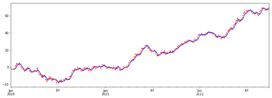
# 画图查看
import matplotlib.pyplot as plt
%matplotlib inline

plt.figure(figsize=(15, 5))

ser_obj.plot(style='r--')
ser_obj.rolling(window=10).mean().plot(style='b')
<matplotlib.axes._subplots.AxesSubplot at 0x22482701630>
print(ser_obj.rolling(window=5, center=True).mean())
2020-01-01          NaN
2020-01-02          NaN
2020-01-03    -1.759677
2020-01-04    -2.380021
2020-01-05    -2.553074
2020-01-06    -2.484760
2020-01-07    -2.397614
2020-01-08    -2.143529
2020-01-09    -2.000231
2020-01-10    -2.009425
2020-01-11    -2.171225
2020-01-12    -2.443878
2020-01-13    -2.631922
2020-01-14    -2.539753
2020-01-15    -2.209591
2020-01-16    -1.449533
2020-01-17    -0.497613
2020-01-18     0.525803
2020-01-19     1.150014
2020-01-20     1.613860
2020-01-21     1.997212
2020-01-22     2.671297
2020-01-23     2.976138
2020-01-24     3.285823
2020-01-25     3.608736
2020-01-26     3.564035
2020-01-27     3.271740
2020-01-28     3.396087
2020-01-29     3.382568
2020-01-30     3.554362
                ...
2022-08-28    67.860530
2022-08-29    68.104397
2022-08-30    68.520018
2022-08-31    68.808258
2022-09-01    68.859020
2022-09-02    68.939447
2022-09-03    69.111310
2022-09-04    68.945411
2022-09-05    68.810430
2022-09-06    68.594266
2022-09-07    68.303743
2022-09-08    67.996121
2022-09-09    67.735381
2022-09-10    67.224599
2022-09-11    66.783246
2022-09-12    66.488297
2022-09-13    66.514767
2022-09-14    66.617468
2022-09-15    66.972475
2022-09-16    67.110751
2022-09-17    67.245906
2022-09-18    67.505485
2022-09-19    67.632520
2022-09-20    67.624951
2022-09-21    68.017344
2022-09-22    68.164661
2022-09-23    68.027393
2022-09-24    68.443821
2022-09-25          NaN
2022-09-26          NaN
Freq: D, Length: 1000, dtype: float64
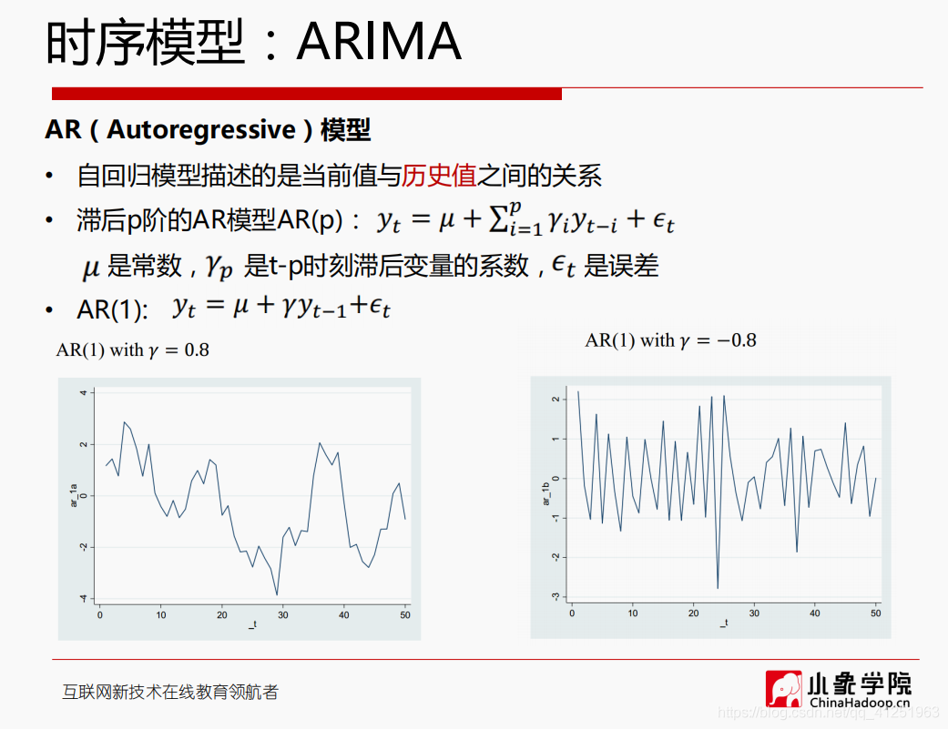
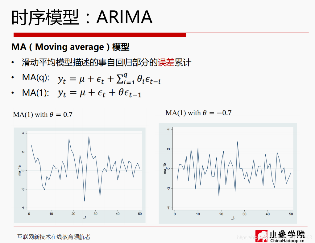
ARIMA模型

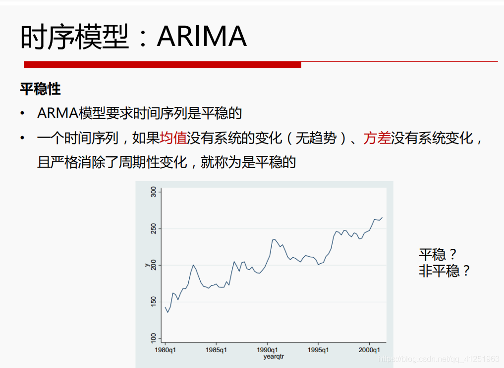
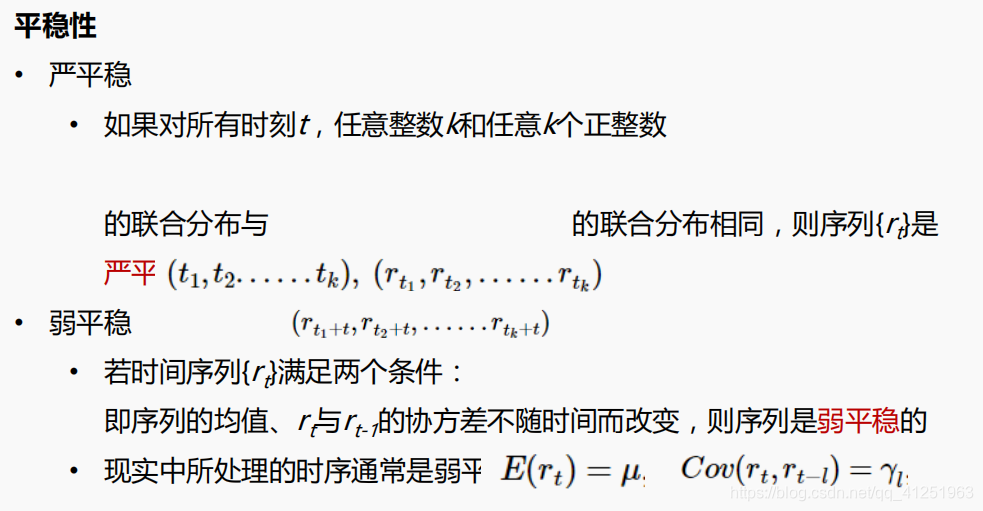
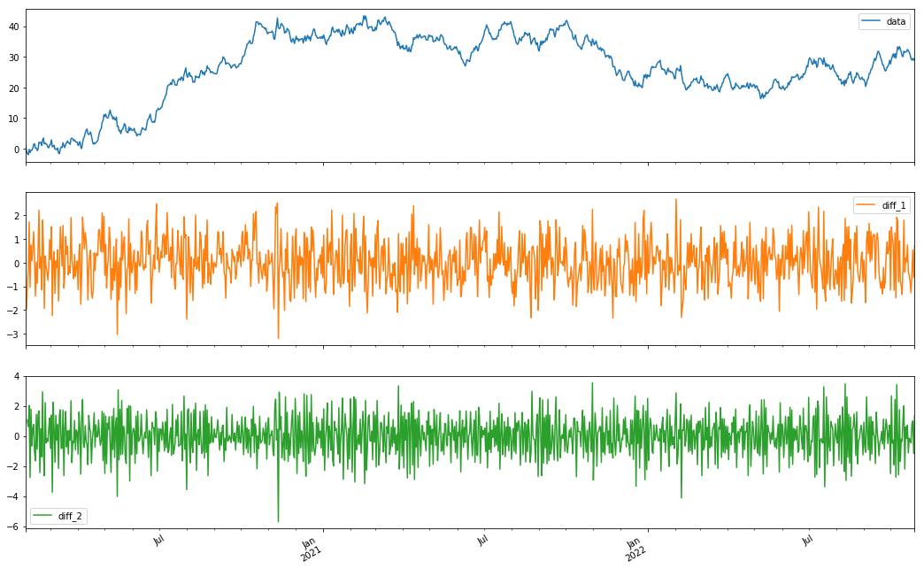
平稳性
import pandas as pd
import numpy as np
import matplotlib.pyplot as plt
%matplotlib inline

# 构造时间时间序列
df_obj = pd.DataFrame(np.random.randn(1000, 1),
                       index=pd.date_range('20200202', periods=1000),
                       columns=['data'])
df_obj['data'] = df_obj['data'].cumsum()
print(df_obj.head())
                data
2020-02-02  1.182594
2020-02-03 -0.774709
2020-02-04 -1.701821
2020-02-05 -2.012117
2020-02-06 -0.292553
# 一阶差分处理
df_obj['diff_1'] = df_obj['data'].diff(1)

# 二阶差分处理
df_obj['diff_2'] = df_obj['diff_1'].diff(1)

# 查看图像
df_obj.plot(subplots=True, figsize=(18, 12))
array([<matplotlib.axes._subplots.AxesSubplot object at 0x0000024168A55A20>,
       <matplotlib.axes._subplots.AxesSubplot object at 0x000002416AAE0BE0>,
       <matplotlib.axes._subplots.AxesSubplot object at 0x000002416AB18FD0>],
      dtype=object)