Performance of Cell-Free Massive MIMO with Rician Fading and Phase Shifts （2）

Performance of Cell-Free Massive MIMO with Rician Fading and Phase Shifts （2）

系统模型

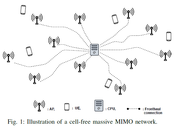
a cell-free Massive MIMO system with

• $M$ APs (single antenna)
• $K$ UEs (single antenna)

如果假设小尺度衰落系数(或相移)之间不存在相关性，那么将每个天线作为一个独立的AP可以直接扩展到多天线的AP情况。
see Cell-free massive mimo systems with multi-antenna users.
However, for a more realistic analysis, single-antenna results can be generalized to multi-antenna case by taking the spatial correlations between antennas into account. It will result in non-diagonal covariance matrices.

The channels are assumed to be constant and frequency-flat in a coherence block of length $\tau_c$ samples (channel uses). The length of each coherence block is determined by the carrier frequency and external factors such as the propagation environment and UE mobility.

The channel $h_{m,k}$ between UE $k$ and the AP $m$ is modeled as
$h_{m,k} = \bar{h}_{m,k}e^{j \varphi_{m,k}} + g_{m,k}$

• Rician fading model: $|h_{m,k}|$ is Rice distributed, but $h_{m,k}$ is not Gaussian distributed (many prior works that neglected the phase shift).
• NLoS propagation small-scale fading: $g_{m,k} \sim \mathcal{CN}(0, \beta_{m,k})$
• variance $\beta_{m,k}$ models large-scale fading, including geometric pathloss and shadowing
• LoS component: $\bar{h}_{m,k} \ge 0$ and $\varphi_{m,k} \sim \mathcal{U}(-\pi, \pi)$

All APs are connected to a central processing unit (CPU) via a fronthaul network that is error free.
The system operates in time division duplex (TDD) mode and the uplink (UL) and DL channels are estimated by exploiting only UL pilot transmission and channel reciprocity.

补充：

• 一个指数分布的概率密度函数是：
  ${\displaystyle f(x;\lambda )=\left\{{\begin{matrix}\lambda e^{-\lambda x}&,\;x\geq 0,\\0&,\;x<0.\end{matrix}}\right.}$

• $r \sim \text{Rayleigh}(\sigma)$ is Rayleigh distributed if ${\displaystyle r={\sqrt {X^{2}+Y^{2}}}}$ where ${\displaystyle X\sim N(0,\sigma ^{2})}$ and ${\displaystyle Y\sim N(0,\sigma ^{2})}$ are independent normal random variables.

• The PDF of the Rayleigh distribution is ${\displaystyle f(x;\sigma )={\frac {x}{\sigma ^{2}}}e^{-x^{2}/(2\sigma ^{2})},\quad x\geq 0,}$
  where $\sigma$ is the scale parameter of the distribution. The CDF is $F(x;\sigma )=1-e^{-x^{2}/(2\sigma ^{2})}$ for $x\in [0,\infty )$.

• if $r = \vert h \vert^2$ has an exponential distribution ${ r \sim \mathrm {Exponential} (\lambda )}$, then let $s={\sqrt {r}}= \vert h \vert$, we have $s \sim \mathrm {Rayleigh} (1/{\sqrt {2\lambda }})$.

  • That is, if $\vert h \vert \sim \mathrm {Rayleigh} ( \sigma )$, we have $\vert h \vert^2 \sim \mathrm {Exponential} ( \frac{1}{2 \sigma^2})$.

• The Rice distribution is a generalization of the Rayleigh distribution: ${\displaystyle \mathrm {Rayleigh} (\sigma )=\mathrm {Rice} (0,\sigma )}$.

• ${\displaystyle R\sim \mathrm {Rice} \left(|\nu |,\sigma \right)}$ has a Rice distribution if $R={\sqrt {X^{2}+Y^{2}}}$ where $X\sim N\left(\nu \cos \theta ,\sigma ^{2}\right)$ and $Y\sim N\left(\nu \sin \theta ,\sigma ^{2}\right)$ are statistically independent normal random variables and $\theta$ is any real number.

• The probability density function is $f(x\mid \nu ,\sigma )={\frac {x}{\sigma ^{2}}}\exp \left({\frac {-(x^{2}+\nu ^{2})}{2\sigma ^{2}}}\right)I_{0}\left({\frac {x\nu }{\sigma ^{2}}}\right)$,
  where $I_0(z)$ is the modified Bessel function of the first kind with order zero.
  The distribution is often also rewritten using the Shape Parameter $K={\frac {\nu ^{2}}{2\sigma ^{2}}}$

• If the random variable $X$ has Rician distribution (unit power in direct and scattered paths), whose PDF is given by
  $f_X(x)=\frac{2x}{\alpha}\text{exp}\left(\frac{-(x^2+\nu^2)}{\alpha}\right)I_0\left(\frac{2x\nu}{\alpha}\right)$

let $\sigma^2 = \alpha/2$, we have $K=\nu^2/\sigma^2$ and
$f_Y(y)=\int_0^\infty dx\ \frac{2x}{\alpha}\text{exp}\left(\frac{-(x^2+\nu^2)}{\alpha}\right)I_0\left(\frac{2x\nu}{\alpha}\right)\delta(y-x^2)$
$= \int_0^\infty dx\ \frac{2x}{\alpha}\text{exp}\left(\frac{-(x^2+\nu^2)} {\alpha}\right)I_0\left(\frac{2x\nu}{\alpha}\right)\frac{\delta(x-\sqrt{y})}{2\sqrt{y}}$

$=\frac{1}{\alpha}\exp\left(\frac{-(y+\nu^2)}{\alpha}\right)I_0\left(\frac{2\nu\sqrt{y}}{\alpha}\right) {=} \frac{1}{2 \sigma^2}\exp\left(\frac{-(y+\nu^2)}{ 2\sigma^2}\right)I_0\left(\frac{2\nu\sqrt{y}}{ 2\sigma^2}\right) ,$

为了简化计算，我们假设 $2 \sigma^2=1$
$\boxed{ \frac{1}{2 \sigma^2}\exp\left(\frac{-(y+\nu^2)}{ 2\sigma^2}\right)I_0\left(\frac{2\nu\sqrt{y}}{ 2\sigma^2}\right) \overset{2\sigma^2 = 1}{\Longrightarrow} \exp\left( -K-y\right)I_0\left(\sqrt{ 4K y} \right)}$
同时我们可得
if $\vert h \vert \sim \mathrm {Rayleigh} ( \sigma )$, we have $\vert h \vert^2 \sim \mathrm {Exponential} ( \frac{1}{2 \sigma^2})$.
$\boxed{ y = \vert h \vert^2 \sim \mathrm {Exponential} ( \frac{1}{2 \sigma^2}) = e^{- y} }$

the modified Bessel functions of the first kind are defined as
$I_{\alpha }(x) = i^{-\alpha }J_{\alpha }(ix)=\sum _{m=0}^{\infty }{\frac {1}{m!\,\Gamma (m+\alpha +1)}}\left({\frac {x}{2}}\right)^{2m+\alpha },$