【数据分析可视化】股票市场分析实战之风险分析

# 基本信息
import numpy as np
import pandas as pd
from pandas import Series, DataFrame

# 股票数据读取
import pandas_datareader as pdr

# 可视化
import matplotlib.pyplot as plt
import seaborn as sns
#%matplotlib inline

# time
from datetime import datetime

# 读取本地数据
alibaba = pd.read_csv('/Users/bennyrhys/Desktop/数据分析可视化-数据集/homework/BABA.csv',index_col=0)
amazon = pd.read_csv('/Users/bennyrhys/Desktop/数据分析可视化-数据集/homework/AMZN.csv',index_col=0)

alibaba.head()

	Open	High	Low	Close	Adj Close	Volume
Date
2015-09-21	65.379997	66.400002	62.959999	63.900002	63.900002	22355100
2015-09-22	62.939999	63.270000	61.580002	61.900002	61.900002	14897900
2015-09-23	61.959999	62.299999	59.680000	60.000000	60.000000	22684600
2015-09-24	59.419998	60.340000	58.209999	59.919998	59.919998	20645700
2015-09-25	60.630001	60.840000	58.919998	59.240002	59.240002	17009100

amazon.head()

	Open	High	Low	Close	Adj Close	Volume
Date
2015-09-21	544.330017	549.780029	539.590027	548.390015	548.390015	3283300
2015-09-22	539.710022	543.549988	532.659973	538.400024	538.400024	3841700
2015-09-23	538.299988	541.210022	534.000000	536.070007	536.070007	2237600
2015-09-24	530.549988	534.559998	522.869995	533.750000	533.750000	3501000
2015-09-25	542.570007	542.799988	521.400024	524.250000	524.250000	4031000

start = datetime(2015,1,1)
company = ['AAPL','GOOG','MSFT','AMZN','FB']
top_tech_df = pdr.get_data_yahoo(company, start=start)['Adj Close']

/Users/bennyrhys/opt/anaconda3/lib/python3.7/site-packages/pandas_datareader/base.py:270: SymbolWarning: Failed to read symbol: 'AAPL', replacing with NaN.
  warnings.warn(msg.format(sym), SymbolWarning)

top_tech_df.head()

Symbols	GOOG	MSFT	AMZN	FB	AAPL
Date
2014-12-31	524.958740	41.587284	310.350006	78.019997	NaN
2015-01-02	523.373108	41.864841	308.519989	78.449997	NaN
2015-01-05	512.463013	41.479866	302.190002	77.190002	NaN
2015-01-06	500.585632	40.871037	295.290009	76.150002	NaN
2015-01-07	499.727997	41.390320	298.420013	76.150002	NaN

# 读取本地数据
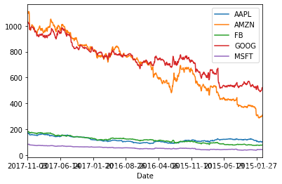
top_tech_df = pd.read_csv('/Users/bennyrhys/Desktop/数据分析可视化-数据集/homework/top5.csv',index_col=0)
top_tech_df.head()

	AAPL	AMZN	FB	GOOG	MSFT
Date
2017-11-03	172.500000	1111.599976	178.919998	1032.479980	84.139999
2017-11-02	168.110001	1094.219971	178.919998	1025.579956	84.050003
2017-11-01	166.889999	1103.680054	182.660004	1025.500000	83.180000
2017-10-31	169.039993	1105.280029	180.059998	1016.640015	83.180000
2017-10-30	166.720001	1110.849976	179.869995	1017.109985	83.889999

# 每日差距
top_tech_dr = top_tech_df.pct_change()
top_tech_dr.head()

	AAPL	AMZN	FB	GOOG	MSFT
Date
2017-11-03	NaN	NaN	NaN	NaN	NaN
2017-11-02	-0.025449	-0.015635	0.000000	-0.006683	-0.001070
2017-11-01	-0.007257	0.008646	0.020903	-0.000078	-0.010351
2017-10-31	0.012883	0.001450	-0.014234	-0.008640	0.000000
2017-10-30	-0.013725	0.005039	-0.001055	0.000462	0.008536

# 画全部
top_tech_df.plot()

<matplotlib.axes._subplots.AxesSubplot at 0x1a2c7be8d0>

# 画局部
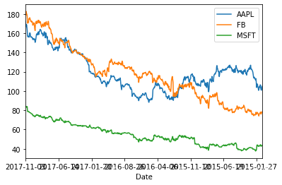
top_tech_df[['AAPL','FB','MSFT']].plot()

<matplotlib.axes._subplots.AxesSubplot at 0x1a2c8506d0>

# 散点图
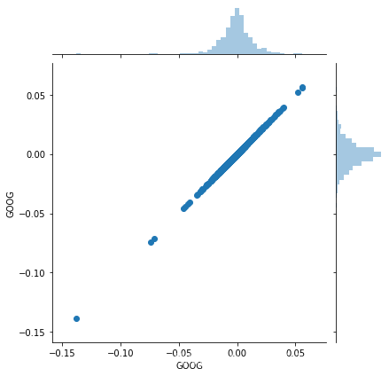
sns.jointplot('GOOG', 'GOOG', top_tech_dr, kind='scatter')

<seaborn.axisgrid.JointGrid at 0x1a27942b90>

# 对比谷歌亚马逊(具有相关性 45度)
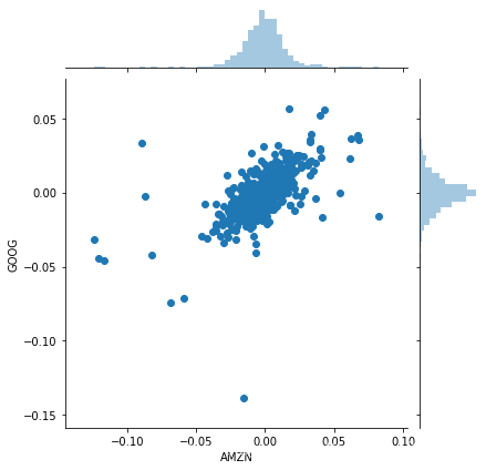
sns.jointplot('AMZN', 'GOOG', top_tech_dr, kind='scatter')

<seaborn.axisgrid.JointGrid at 0x1a2794aa90>

# 相关性相对小（上移 且 宽）
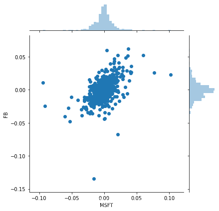
sns.jointplot('MSFT', 'FB', top_tech_dr, kind='scatter')

<seaborn.axisgrid.JointGrid at 0x1a2d45af10>

# 矩阵散点图(可以看到谷歌和亚马逊最接近)
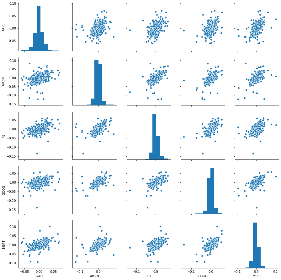
sns.pairplot(top_tech_dr.dropna())

<seaborn.axisgrid.PairGrid at 0x1a2d694710>

# 分位数（涉及数学比较多）
# 可以理解为误差百分比,48%-0.0001447090809730694
top_tech_dr['AAPL'].quantile(0.52)

-0.0001447090809730694

top_tech_dr['AAPL'].quantile(0.05)

-0.022946394303717855

# 唯品会的趋势
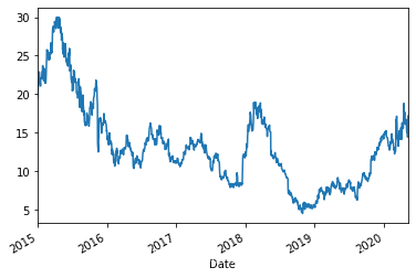
vips = pdr.get_data_yahoo('VIPS', start=start)['Adj Close']
vips.plot()

<matplotlib.axes._subplots.AxesSubplot at 0x1a32a77e50>

vips.pct_change().quantile(0.2)

-0.023114020115947723