前三篇文章，讨论了单变量、多变量和多步时间序列预测。对于不同的问题，可以使用不同类型的LSTM模型，例如Vanilla、Stacked、Bidirectional、CNN-LSTM、Conv LSTM模型。这也适用于涉及多变量和多时间步预测的时间序列预测问题，但可能更具挑战性。本文将介绍多变量多时间步预测LSTM模型，主要内容如下：

多变量输入多时间步预测输出模型（Multiple Input Multi-step Output）
多并行输入多时间步预测输出模型（Multiple Parallel Input and Multi-step Output）

【Part1】如何开发LSTM实现时间序列预测详解 01 Univariate LSTM
【Part2】如何开发LSTM实现时间序列预测详解 02 Multivariate LSTM
【Part3】如何开发LSTM实现时间序列预测详解 03 Multi-step LSTM

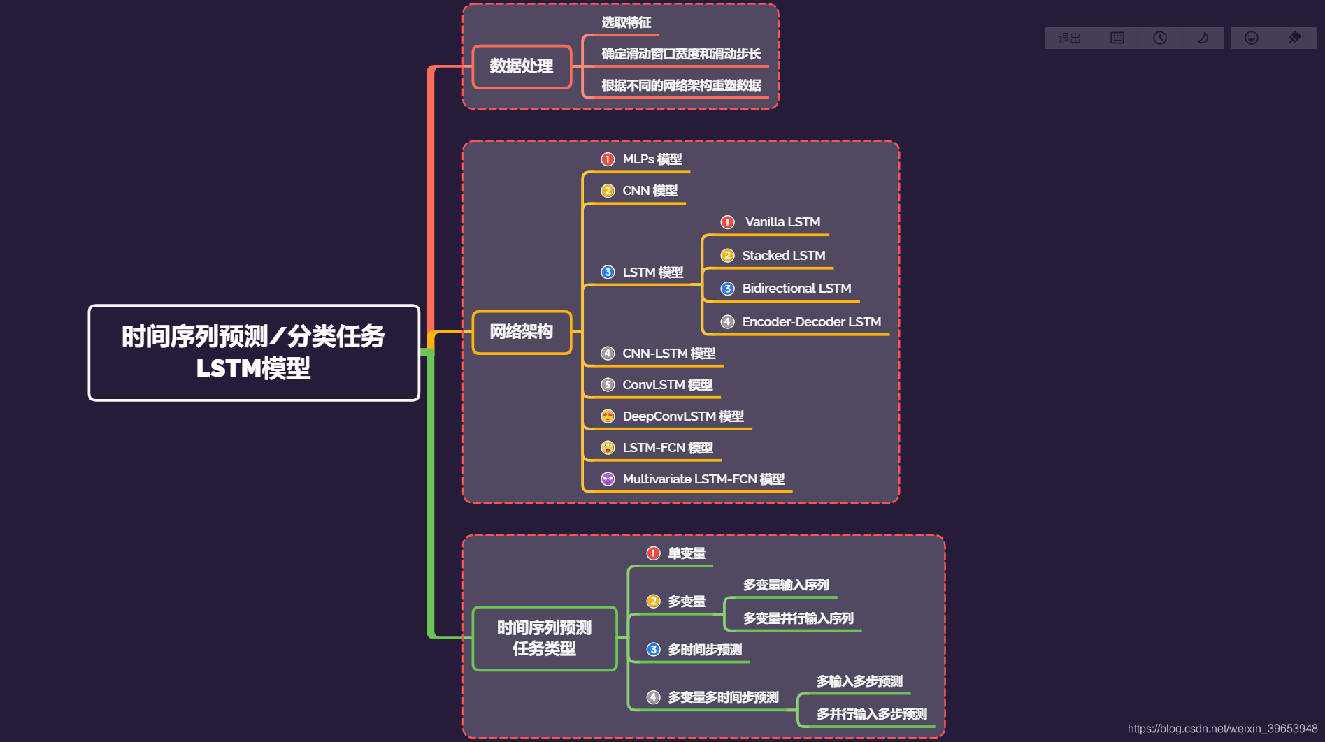
本文是LSTM时间序列预测任务的第四篇。LSTM用在时间序列的问题上，主要由两类任务：一类是时间序列预测，另一类是时间序列分类，这四篇文章介绍的是时间序列预测；关于时间序列分类以后的文章会介绍。看一下思维导图：
在这里插入图片描述
四篇文章的行文顺序是按照时间序列预测的任务类型来划分的，本文介绍的内容是多变量多时间步预测任务。

4.1 多变量输入多时间步预测（Multiple Input Multi-Step Output）
4.2 多并行输入多时间步预测（Multiple Parallel Input and Multi-step Output）
4.3 完整代码

4.3.1 数据处理和模型定义
4.3.2 实例化代码
4.3.3 数据处理、转化过程、模型结构等信息输出

总结

4. 多变量多时间步预测输出模型

4.1 多变量输入多时间步预测（Multiple Input Multi-Step Output）

在多变量时间序列预测问题中，输出序列是独立的，但依赖于输入序列，输出序列有多个时间步的预测输出值。考虑前三篇文章中使用的多元时间序列：

[[ 10 15 25]
[ 20 25 45]
[ 30 35 65]
[ 40 45 85]
[ 50 55 105]
[ 60 65 125]
[ 70 75 145]
[ 80 85 165]
[ 90 95 185]]

假设我们使用两个输入时间序列中前两个特征采样值来预测后一个特征的输出时间序列的两个时间步的采样点的值，那么我们可以将上述序列数据划分成样本，划分结果如下，为了增加文章可读性，此处不放出代码，仅贴出划分结果，方便理解，代码会在完整代码中给出：

[[10 15]
[20 25]
[30 35]] [65 85]
[[20 25]
[30 35]
[40 45]] [ 85 105]
[[30 35]
[40 45]
[50 55]] [105 125]
[[40 45]
[50 55]
[60 65]] [125 145]
[[50 55]
[60 65]
[70 75]] [145 165]
[[60 65]
[70 75]
[80 85]] [165 185]

训练样本的输入数据形状和期望输出的尺寸分别为：

(6, 3, 2),(6, 2)

划分完数据后，接下来定义LSTM模型。可以使用向量输出模型或编码器-解码器模型。此处使用堆叠LSTM实现，模型定义如下：

model = Sequential()
model.add(LSTM(100, activation='relu', return_sequences=True, input_shape=(sw_width, n_features)))
model.add(LSTM(100, activation='relu'))
model.add(Dense(pred_length))
model.compile(optimizer='adam', loss='mse')

完整代码在文末。

4.2 多并行输入多时间步预测（Multiple Parallel Input and Multi-step Output）

还是通过上文提到的序列化数据来说明多并行输入多步输出是怎么回事，一看就明白了。

扫描二维码关注公众号，回复： 10954249 查看本文章

[[ 10 15 25]
[ 20 25 45]
[ 30 35 65]
[ 40 45 85]
[ 50 55 105]
[ 60 65 125]
[ 70 75 145]
[ 80 85 165]
[ 90 95 185]]

由以上序列，我们取第一个样本进行说明。

输入的训练样本数据（X）为：

10, 15, 25
20, 25, 45
30, 35, 65

期望的预测输出（y）为：

40, 45, 85
50, 55, 105

将整个序列数据进行划分：

[[10 15 25]
[20 25 45]
[30 35 65]] [[ 40 45 85]
[ 50 55 105]]
[[20 25 45]
[30 35 65]
[40 45 85]] [[ 50 55 105]
[ 60 65 125]]
[[ 30 35 65]
[ 40 45 85]
[ 50 55 105]] [[ 60 65 125]
[ 70 75 145]]
[[ 40 45 85]
[ 50 55 105]
[ 60 65 125]] [[ 70 75 145]
[ 80 85 165]]
[[ 50 55 105]
[ 60 65 125]
[ 70 75 145]] [[ 80 85 165]
[ 90 95 185]]

划分后，训练样本的输入数据形状和期望预测输出的形状为：

(5, 3, 3) (5, 2, 3)

其中 (5, 3, 3) 中的 “5” 表示样本数（samples），“3” 表示滑动窗口的宽度（sw_width），最后一个维度的 “3” 表示特征数（features）；(5, 2, 3) 中的 “5” 表示样本数（samples），“2” 表示预测序列的长度，“3” 表示每个序列包含的特征数。

样本划分好之后，我们就来训练模型。此处使用编码器-解码器模型来训练多并行输入多时间步预测输出的数据。

以上两个模型的完整代码如下。

4.3 完整代码

比较难理解的地方做了注释，数据处理转化过程、模型信息都打印出来了，应该很容易理解。

4.3.1 数据处理和模型定义

import numpy as np
from tensorflow.keras.models import Sequential, Model
from tensorflow.keras.layers import Dense, LSTM, Flatten
from tensorflow.keras.layers import RepeatVector, TimeDistributed

def mock_seq(seq1, seq2):
    '''
    构造虚拟序列数据
    实现将多个单列序列数据构造成类似于实际数据的列表的格式
    '''
    seq1 = np.array(seq1)
    seq2 = np.array(seq2)
    seq3 = np.array([seq1[i]+seq2[i] for i in range(len(seq1))])
    
    seq1 = seq1.reshape((len(seq1), 1))
    seq2 = seq2.reshape((len(seq2), 1))
    seq3 = seq3.reshape((len(seq3), 1))
    
    # 对于二维数组，沿第二个维度堆叠，相当于列数增加；可以想象成往书架里一本一本的摆书
    dataset = np.hstack((seq1, seq2, seq3))
    
    return dataset
        
    
class MultivariateMultiStepModels:
    '''
    多变量多时间步预测LSTM模型
    '''
    def __init__(self, train_seq, test_seq, sw_width, pred_length, epochs_num, verbose_set): 
        '''
        初始化变量和参数
        '''
        self.train_seq = train_seq
        self.test_seq = test_seq
        self.sw_width = sw_width
        self.pred_length = pred_length
        
        self.epochs_num = epochs_num
        self.verbose_set = verbose_set
        
        self.X, self.y = [], []     
        
    def split_sequence_multi_output(self):
        '''
        该函数实现多输入序列数据的样本划分
        '''
        for i in range(len(self.train_seq)):
            # 找到最后一个元素的索引，因为for循环中i从1开始，切片索引从0开始，切片区间前闭后开，所以不用减去1；
            end_index = i + self.sw_width
            # 找到输出预测序列的最大索引，便于截取数据，因为i从1开始，切片索引从0开始，所以需要减去1；
            out_end_index = end_index + self.pred_length - 1
            # 如果最后一个滑动窗口中的最后一个元素的索引大于序列中最后一个元素的索引则丢弃该样本；
            # 这里len(self.sequence)没有减去1的原因是：保证最后一个元素的索引恰好等于序列数据索引时，能够截取到样本；
            if out_end_index > len(self.train_seq) :
                break
                
            # 实现以滑动步长为1（因为是for循环），窗口宽度为self.sw_width的滑动步长取值；
            # [i:end_index, :-1] 截取第i行到第end_index-1行、除最后一列之外的列的数据；
            # [end_index-1:out_end_index, -1] 截取第end_index-1行到第out_end_index行、最后一列的数据；
            seq_x, seq_y = self.train_seq[i:end_index, :-1], self.train_seq[end_index-1:out_end_index, -1]
            self.X.append(seq_x)
            self.y.append(seq_y)
            
        self.X, self.y = np.array(self.X), np.array(self.y)
        self.features = self.X.shape[2]
        self.test_seq = self.test_seq.reshape((1, self.sw_width, self.test_seq.shape[1]))

        for i in range(len(self.X)):
            print(self.X[i], self.y[i])
        
        print('X:\n{}\ny:\n{}\ntest_seq:\n{}\n'.format(self.X, self.y, self.test_seq))
        print('X.shape:{}, y.shape:{}, test_seq.shape:{}\n'.format(self.X.shape, self.y.shape, self.test_seq.shape))
        
        return self.X, self.y, self.features, self.test_seq
    
    def split_sequence_parallel(self):
        '''
        该函数实现多输入序列数据的样本划分
        注意切片区间的选取！其实记住前闭后开区间就很好理解了。
        '''
        for i in range(len(self.train_seq)):
            end_index = i + self.sw_width
            out_end_index = end_index + self.pred_length
            if out_end_index > len(self.train_seq) :
                break
                
            # [i:end_index, :] 截取第i行到第end_index-1行、所有列的数据；
            # [end_index:out_end_index, :] 截取第end_index行到第out_end_index行、所有列的数据；
            seq_x, seq_y = self.train_seq[i:end_index, :], self.train_seq[end_index:out_end_index, :]
            self.X.append(seq_x)
            self.y.append(seq_y)
            
        self.X, self.y = np.array(self.X), np.array(self.y)
        self.features = self.X.shape[2]
        self.test_seq = self.test_seq.reshape((1, self.sw_width, self.test_seq.shape[1]))

        for i in range(len(self.X)):
            print(self.X[i], self.y[i])
        
        print('X:\n{}\ny:\n{}\ntest_seq:\n{}\n'.format(self.X, self.y, self.test_seq))
        print('X.shape:{}, y.shape:{}, test_seq.shape:{}\n'.format(self.X.shape, self.y.shape, self.test_seq.shape))
        
        return self.X, self.y, self.features, self.test_seq    
    
    def stacked_lstm(self):
        model = Sequential()
        model.add(LSTM(100, activation='relu', return_sequences=True, 
                       input_shape=(self.sw_width, self.features)))
        model.add(LSTM(100, activation='relu'))
        model.add(Dense(units=self.pred_length))
        model.compile(optimizer='adam', loss='mse', metrics=['accuracy'])
        print(model.summary())
        
        history = model.fit(self.X, self.y, epochs=self.epochs_num, verbose=self.verbose_set)
        print('\ntrain_acc:%s'%np.mean(history.history['accuracy']), '\ntrain_loss:%s'%np.mean(history.history['loss']))
        print('yhat:%s'%(model.predict(self.test_seq)),'\n-----------------------------')
        
    def encoder_decoder_lstm(self):
        model = Sequential()
        model.add(LSTM(200, activation='relu',
                       input_shape=(self.sw_width, self.features)))
        model.add(RepeatVector(self.pred_length))
        model.add(LSTM(200, activation='relu', return_sequences=True))
        model.add(TimeDistributed(Dense(self.features)))
        model.compile(optimizer='adam', loss='mse', metrics=['accuracy'])
        print(model.summary())
        
        history = model.fit(self.X, self.y, epochs=self.epochs_num, verbose=self.verbose_set)
        print('\ntrain_acc:%s'%np.mean(history.history['accuracy']), '\ntrain_loss:%s'%np.mean(history.history['loss']))
        print('yhat:%s'%(model.predict(self.test_seq)),'\n-----------------------------')

4.3.2 实例化代码

if __name__ == '__main__':
    
    orig_seq1 = [10, 20, 30, 40, 50, 60, 70, 80, 90]
    orig_seq2 = [15, 25, 35, 45, 55, 65, 75, 85, 95]
    train_seq = mock_seq(orig_seq1, orig_seq2)
    
    test_seq_multi = np.array([[80, 85], [90, 95], [100, 105]])
    test_seq_paral = np.array([[60, 65, 125], [70, 75, 145], [80, 85, 165]])
    
    sliding_window_width = 3
    predict_length = 2
    epochs_num = 200
    verbose_set = 0
    
    print('-------以下为 【多输入多时间步预测输出 LSTM 模型】 相关信息------')
    MultivariateMultiStepLSTM = MultivariateMultiStepModels(train_seq, test_seq_multi, sliding_window_width, predict_length,
                                                            epochs_num, verbose_set)
    MultivariateMultiStepLSTM.split_sequence_multi_output()
    MultivariateMultiStepLSTM.stacked_lstm()
    
    print('-------以下为 【并行输入多时间步预测输出 LSTM 模型】 相关信息------')
    MultivariateMultiStepLSTM = MultivariateMultiStepModels(train_seq, test_seq_paral, sliding_window_width, predict_length,
                                                            epochs_num, verbose_set)
    MultivariateMultiStepLSTM.split_sequence_parallel()
    MultivariateMultiStepLSTM.encoder_decoder_lstm()

4.3.3 数据处理、转化过程、模型结构等信息输出

-------以下为 【多输入多时间步预测输出 LSTM 模型】 相关信息------
[[10 15]
 [20 25]
 [30 35]] [65 85]
[[20 25]
 [30 35]
 [40 45]] [ 85 105]
[[30 35]
 [40 45]
 [50 55]] [105 125]
[[40 45]
 [50 55]
 [60 65]] [125 145]
[[50 55]
 [60 65]
 [70 75]] [145 165]
[[60 65]
 [70 75]
 [80 85]] [165 185]
X:
[[[10 15]
  [20 25]
  [30 35]]

 [[20 25]
  [30 35]
  [40 45]]

 [[30 35]
  [40 45]
  [50 55]]

 [[40 45]
  [50 55]
  [60 65]]

 [[50 55]
  [60 65]
  [70 75]]

 [[60 65]
  [70 75]
  [80 85]]]
y:
[[ 65  85]
 [ 85 105]
 [105 125]
 [125 145]
 [145 165]
 [165 185]]
test_seq:
[[[ 80  85]
  [ 90  95]
  [100 105]]]

X.shape:(6, 3, 2), y.shape:(6, 2), test_seq.shape:(1, 3, 2)

Model: "sequential"
_________________________________________________________________
Layer (type)                 Output Shape              Param #   
=================================================================
lstm (LSTM)                  (None, 3, 100)            41200     
_________________________________________________________________
lstm_1 (LSTM)                (None, 100)               80400     
_________________________________________________________________
dense (Dense)                (None, 2)                 202       
=================================================================
Total params: 121,802
Trainable params: 121,802
Non-trainable params: 0
_________________________________________________________________
None

train_acc:0.8641666 
train_loss:1499.5305340608954
yhat:[[207.57896 231.91385]] 
-----------------------------
-------以下为 【并行输入多时间步预测输出 LSTM 模型】 相关信息------
[[10 15 25]
 [20 25 45]
 [30 35 65]] [[ 40  45  85]
 [ 50  55 105]]
[[20 25 45]
 [30 35 65]
 [40 45 85]] [[ 50  55 105]
 [ 60  65 125]]
[[ 30  35  65]
 [ 40  45  85]
 [ 50  55 105]] [[ 60  65 125]
 [ 70  75 145]]
[[ 40  45  85]
 [ 50  55 105]
 [ 60  65 125]] [[ 70  75 145]
 [ 80  85 165]]
[[ 50  55 105]
 [ 60  65 125]
 [ 70  75 145]] [[ 80  85 165]
 [ 90  95 185]]
X:
[[[ 10  15  25]
  [ 20  25  45]
  [ 30  35  65]]

 [[ 20  25  45]
  [ 30  35  65]
  [ 40  45  85]]

 [[ 30  35  65]
  [ 40  45  85]
  [ 50  55 105]]

 [[ 40  45  85]
  [ 50  55 105]
  [ 60  65 125]]

 [[ 50  55 105]
  [ 60  65 125]
  [ 70  75 145]]]
y:
[[[ 40  45  85]
  [ 50  55 105]]

 [[ 50  55 105]
  [ 60  65 125]]

 [[ 60  65 125]
  [ 70  75 145]]

 [[ 70  75 145]
  [ 80  85 165]]

 [[ 80  85 165]
  [ 90  95 185]]]
test_seq:
[[[ 60  65 125]
  [ 70  75 145]
  [ 80  85 165]]]

X.shape:(5, 3, 3), y.shape:(5, 2, 3), test_seq.shape:(1, 3, 3)

Model: "sequential_1"
_________________________________________________________________
Layer (type)                 Output Shape              Param #   
=================================================================
lstm_2 (LSTM)                (None, 200)               163200    
_________________________________________________________________
repeat_vector (RepeatVector) (None, 2, 200)            0         
_________________________________________________________________
lstm_3 (LSTM)                (None, 2, 200)            320800    
_________________________________________________________________
time_distributed (TimeDistri (None, 2, 3)              603       
=================================================================
Total params: 484,603
Trainable params: 484,603
Non-trainable params: 0
_________________________________________________________________
None

train_acc:1.0 
train_loss:499.6571237371396
yhat:[[[ 90.40701  96.32832 186.49251]
  [100.81339 104.66335 205.89095]]] 
-----------------------------

总结

结合四篇文章的讲解和代码示例，相信你已经对LSTM实现时间序列预测任务有了比较深的理解。这四篇文章主要讲了如下内容：

如何开发用于单变量（一个特征）时间序列预测LSTM模型；
如何开发用于多变量（多个特征）时间序列预测的LSTM模型；
如何开发用于多时间步输出时间序列预测的LSTM模型。

再来看一下思维导图，总结这四篇文章，关于LSTM处理时间序列预测或者分类的模型还有 DeepConvLSTM、LSTM-FCN、Multivariate LSTM-FCN…等等，本文没有提及，包括时间序列分类任务也没有提及，以后的文章会专门写，包括相关论文和代码以及使用真实数据集的实际应用。
在这里插入图片描述