时间序列预测18：ConvLSTM 实现用电量/发电量预测

接上文，本文介绍了ConvLSTM模型实现用电量/发电量预测。

---

LSTM 处理用电量/发电量预测任务的文章：

【Part1】Encoder-Decoder LSTM 模型 实现用电量/发电量预测
【Part2】CNN-LSTM 模型 实现用电量/发电量预测
【Part3】本文

---

---

1. ConvLSTM

1.1 CNN 模型

CNN-LSTM方法的进一步扩展是执行CNN的卷积（例如CNN如何读取输入序列数据）作为LSTM的一部分用于每个时间步。这种组合称为ConvLSTM，与CNN-LSTM一样，它也用于时空数据。与直接读取数据以计算内部状态和状态转换的LSTM不同，与解释CNN模型输出的CNN-LSTM也不同，ConvLSTM直接使用卷积作为读取LSTM单元输入的一部分。Keras库提供了ConvLSTM2D类，该类支持二维数据的ConvLSTM模型。它可以配置为一维多变量时间序列预测。默认情况下，ConvLSTM2D类要求输入数据的形状为：[samples，timesteps，rows，cols，channels]。

其中数据的每个时间步均定义为（行×列）数据点的图像。我们正在处理总功耗的一维序列，如果我们假设我们使用两周的数据作为输入，则行为1，列为14。ConvLSTM将一次读取这些数据，即LSTM读取一个14天的时间步长，并在这些时间步长上进行卷积。

在我们的任务中，可以将14天分成两个子序列，每个子序列的长度为7天。然后，ConvLSTM可以读取两个时间步长，并对每个时间步长中的7天数据执行CNN处理。因此，对于此问题的选定框架，ConvLSTM2D的输入shape为：[n，2，1，7，1]。参数说明：

• 样本（samples）：n，表示训练数据集中的样本数。
• 时间步长（timesteps）：2，表示将一个窗口宽度为14天的采样数据分为两个子序列。
• 行（rows）：1，表示每个子序列的一维形状，即有多少行。
• 列（cols）：7，表示每个子序列，有多少列。
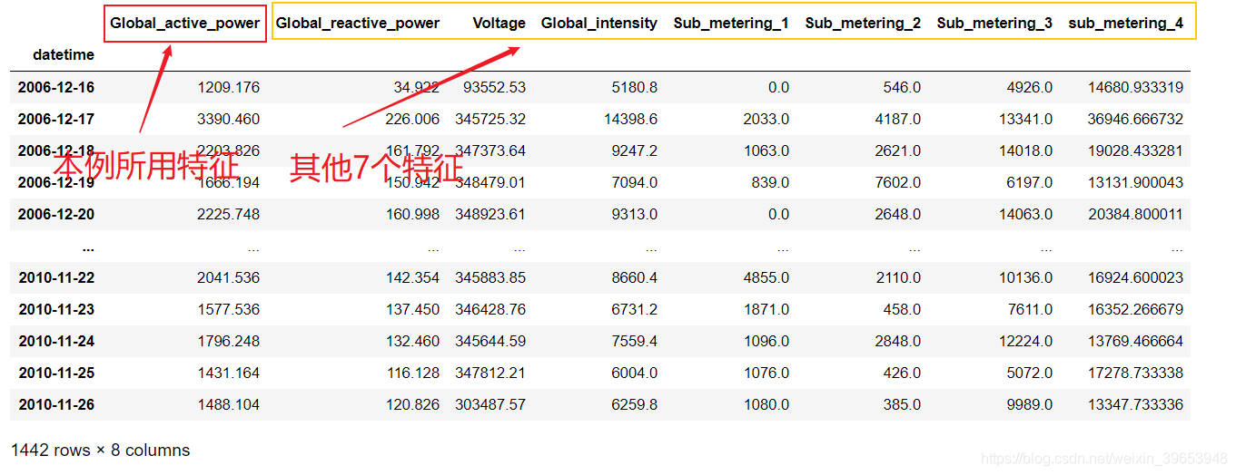
• 通道（channels）：1，在图像识别任务中的概念，通道数。在时间序列预测任务中其实就是特征数（features），这个概念在之前的文章中反复提及强调。因为本例的业务需求是通过日总功耗来预测下周的日总功耗，所以通道数（特征数）为1，即代表日总功耗。如果要添加其他的特征，这个尺寸要做相应改变。再看下数据集情况，就一目了然了。
  
  还可以探索其他配置，例如使用前21天的总功耗作为输入，并将其分为3个子序列，和/或提供所有八个功能或通道作为输入。ConvLSTM2D的数据输入要求必须将训练数据集重塑为[样本，时间步长，行，列，通道]（[samples, timesteps, rows, cols, channels]）的结构。对比CNN-LSTM完整代码，需要在此基础上做如下修改：

1. 重塑训练样本的shape：

train_x = train_x.reshape((train_x.shape[0], n_steps, 1, n_length, n_features))

2. 设定ConvLSTM模型的输入尺寸参数：

model.add(ConvLSTM2D(filters=64, kernel_size=(1,3), activation='relu',input_shape=(sw_width, 1, n_length, n_features)))
model.add(Flatten())

3. 重塑测试样本的shape：

input_x = input_x.reshape((1, sw_width, 1, n_length, 1))

---

1.2 完整代码

import numpy as np
import pandas as pd
import matplotlib.pyplot as plt

# 设置中文显示
plt.rcParams['font.sans-serif'] = ['Microsoft JhengHei']
plt.rcParams['axes.unicode_minus'] = False

import math
import sklearn.metrics as skm
from tensorflow.keras.models import Sequential
from tensorflow.keras.layers import LSTM, Dense
from tensorflow.keras.layers import RepeatVector, TimeDistributed
from tensorflow.keras.layers import ConvLSTM2D


def split_dataset(data):
    '''
    该函数实现以周为单位切分训练数据和测试数据
    '''
    # data为按天的耗电量统计数据，shape为(1442, 8)
    # 测试集取最后一年的46周（322天）数据，剩下的159周（1113天）数据为训练集，以下的切片实现此功能。
    train, test = data[1:-328], data[-328:-6]
    train = np.array(np.split(train, len(train)/7)) # 将数据划分为按周为单位的数据
    test = np.array(np.split(test, len(test)/7))
    return train, test

def evaluate_forecasts(actual, predicted):
    '''
    该函数实现根据预期值评估一个或多个周预测损失
    思路：统计所有单日预测的 RMSE
    '''
    scores = list()
    for i in range(actual.shape[1]):
        mse = skm.mean_squared_error(actual[:, i], predicted[:, i])
        rmse = math.sqrt(mse)
        scores.append(rmse)
    
    s = 0 # 计算总的 RMSE
    for row in range(actual.shape[0]):
        for col in range(actual.shape[1]):
            s += (actual[row, col] - predicted[row, col]) ** 2
    score = math.sqrt(s / (actual.shape[0] * actual.shape[1]))
    print('actual.shape[0]:{}, actual.shape[1]:{}'.format(actual.shape[0], actual.shape[1]))
    return score, scores

def summarize_scores(name, score, scores):
    s_scores = ', '.join(['%.1f' % s for s in scores])
    print('%s: [%.3f] %s\n' % (name, score, s_scores))
    
def sliding_window(train, sw_width=7, n_out=7, in_start=0):
    '''
    该函数实现窗口宽度为7、滑动步长为1的滑动窗口截取序列数据
    '''
    data = train.reshape((train.shape[0] * train.shape[1], train.shape[2])) # 将以周为单位的样本展平为以天为单位的序列
    X, y = [], []
    
    for _ in range(len(data)):
        in_end = in_start + sw_width
        out_end = in_end + n_out
        
        # 保证截取样本完整，最大元素索引不超过原序列索引，则截取数据；否则丢弃该样本
        if out_end < len(data):
            # 训练数据以滑动步长1截取
            train_seq = data[in_start:in_end, 0]
            train_seq = train_seq.reshape((len(train_seq), 1))
            X.append(train_seq)
            y.append(data[in_end:out_end, 0])
        in_start += 1
        
    return np.array(X), np.array(y)

def conv_lstm_model(train, sw_width, n_steps, n_length, in_start=0, verbose_set=0, epochs_num=20, batch_size_set=4):
    '''
    该函数定义 Encoder-Decoder LSTM 模型
    '''
    train_x, train_y = sliding_window(train, sw_width, in_start=0)
    n_timesteps, n_features, n_outputs = train_x.shape[1], train_x.shape[2], train_y.shape[1]
    
    train_x = train_x.reshape((train_x.shape[0], n_steps, 1, n_length, n_features))
    train_y = train_y.reshape((train_y.shape[0], train_y.shape[1], 1))
    
    model = Sequential()
    model.add(ConvLSTM2D(filters=64, kernel_size=(1,3), activation='relu',
                         input_shape=(n_steps, 1, n_length, n_features)))
    model.add(Flatten())
    model.add(RepeatVector(n_outputs))
    model.add(LSTM(200, activation='relu', return_sequences=True))
    model.add(TimeDistributed(Dense(100, activation='relu')))
    model.add(TimeDistributed(Dense(1)))
    
    model.compile(loss='mse', optimizer='adam', metrics=['accuracy'])
    print(model.summary())
    
    model.fit(train_x, train_y,
              epochs=epochs_num, batch_size=batch_size_set, verbose=verbose_set)
    return model

def forecast(model, pred_seq, sw_width, n_length, n_steps):
    '''
    该函数实现对输入数据的预测
    '''
    data = np.array(pred_seq)
    data = data.reshape((data.shape[0]*data.shape[1], data.shape[2]))
    
    input_x = data[-sw_width:, 0] # 获取输入数据的最后一周的数据
    input_x = input_x.reshape((1, n_steps, 1, n_length, 1))
    
    yhat = model.predict(input_x, verbose=0) # 预测下周数据
    yhat = yhat[0] # 获取预测向量
    return yhat

def evaluate_model(model, train, test, sd_width, n_length, n_steps):
    '''
    该函数实现模型评估
    '''
    history_fore = [x for x in train]
    predictions = list() # 用于保存每周的前向验证结果；
    for i in range(len(test)):
        yhat_sequence = forecast(model, history_fore, sd_width, n_length, n_steps) # 预测下周的数据
        predictions.append(yhat_sequence) # 保存预测结果
        history_fore.append(test[i, :]) # 得到真实的观察结果并添加到历史中以预测下周
    
    predictions = np.array(predictions) # 评估一周中每天的预测结果
    score, scores = evaluate_forecasts(test[:, :, 0], predictions)
    return score, scores

def model_plot(score, scores, days, name):
    '''
    该函数实现绘制RMSE曲线图
    '''
    plt.figure(figsize=(8,6), dpi=150)
    plt.plot(days, scores, marker='o', label=name)
    plt.grid(linestyle='--', alpha=0.5)
    plt.ylabel(r'$RMSE$', size=15)
    plt.title('Conv-LSTM 模型预测结果',  size=18)
    plt.legend()
    plt.show()
    
def main_run(dataset, sw_width, days, name, in_start, verbose, epochs, batch_size, n_steps, n_length):
    '''
    主函数：数据处理、模型训练流程
    '''
    # 划分训练集和测试集
    train, test = split_dataset(dataset.values)
    # 训练模型
    model = conv_lstm_model(train, sw_width,  n_steps, n_length, in_start, verbose_set=0, epochs_num=20, batch_size_set=4)
    # 计算RMSE
    score, scores = evaluate_model(model, train, test, sw_width, n_length, n_steps)
    # 打印分数
    summarize_scores(name, score, scores)
    # 绘图
    model_plot(score, scores, days, name)
    
    print('------头发不够，帽子来凑-----')
    
    
if __name__ == '__main__':
    
    dataset = pd.read_csv('household_power_consumption_days.csv', header=0, 
                   infer_datetime_format=True, engine='c',
                   parse_dates=['datetime'], index_col=['datetime'])
    
    days = ['sun', 'mon', 'tue', 'wed', 'thr', 'fri', 'sat']
    name = 'Conv-LSTM'
    
    # 定义序列的数量和长度
    '''
    n_steps：子序列划分的数量，本例为2，将14天的数据划分为两个7的子序列；
    n_length：子序列每行的元素数，即列数。
    '''
    n_steps, n_length = 2, 7
    
    sliding_window_width= n_length * n_steps
    input_sequence_start=0
    
    epochs_num=20
    batch_size_set=16
    verbose_set=0
    
    
    main_run(dataset, sliding_window_width, days, name, input_sequence_start,
             verbose_set, epochs_num, batch_size_set, n_steps, n_length)

输出：

Model: "sequential_12"
_________________________________________________________________
Layer (type)                 Output Shape              Param #   
=================================================================
conv_lst_m2d_2 (ConvLSTM2D)  (None, 1, 5, 64)          50176     
_________________________________________________________________
flatten_3 (Flatten)          (None, 320)               0         
_________________________________________________________________
repeat_vector_8 (RepeatVecto (None, 7, 320)            0         
_________________________________________________________________
lstm_16 (LSTM)               (None, 7, 200)            416800    
_________________________________________________________________
time_distributed_16 (TimeDis (None, 7, 100)            20100     
_________________________________________________________________
time_distributed_17 (TimeDis (None, 7, 1)              101       
=================================================================
Total params: 487,177
Trainable params: 487,177
Non-trainable params: 0
_________________________________________________________________
None
actual.shape[0]:46, actual.shape[1]:7
Conv-LSTM: [382.156] 391.3, 386.4, 340.5, 388.9, 364.4, 309.1, 473.6

运行示例总结测试集的性能。实验表明，使用两个卷积层使模型比仅使用单个层更稳定。可以看到，在这种情况下，该模型表现较好，总体RMSE得分约为382千瓦。

---

扩展

• 输入大小：探索模型的输入天数，例如3天，21天，30天等等。
• 模型调整：调整模型的结构和超参数，并进一步提升模型性能。
• 数据缩放：探索是否可以使用数据缩放（例如标准化和规范化）来改善LSTM模型的性能。
• 学习诊断：使用诊断（例如训练的学习曲线和验证损失以及均方误差）来帮助调整LSTM模型的结构和超参数。

---

总结

三篇文章介绍了如何开发LSTM来进行家庭用电量的多步时间序列预测。主要有以下内容：

• 如何开发和评估用于多步时间序列预测的单变量和多变量Encoder-Decoder LSTM 模型。
• 如何开发和评估用于多步时间序列预测的CNN-LSTM Encoder-Decoder 模型。
• 如何开发和评估用于多步时间序列预测的ConvLSTM Encoder-Decoder 模型。

---

关于时间序列预测用电量预测任务先告一段落，下篇文章开始介绍时间序列分类任务，比如人类行为识别，车辆驾驶行为识别。

---