【LSTM】入门天气数据集实验--理解长短期记忆模型

一、简介

LSTM（Long short-Term Memory）是一种 RNN 特殊的类型，可以学习长期依赖信息。

LSTM 由Hochreiter & Schmidhuber (1997)提出，并在近期被Alex Graves进行了改良和推广。在很多问题，LSTM 都取得相当巨大的成功，并得到了广泛的使用。

1.与HMM比较

隐马尔可夫模型HMM简介

HMM是最早期的序列预测的算法：

“HMM“和”“RNN”的关系就像“桌子”和“板子”，不是一回事，但也不是完全没关系。

在机器学习分类中，“HMM”被划分为“经典机器学习算法”，“RNN”则为“经典的深度学习模型”。

RNN与HMM的本质区别是RNN没有马尔科夫假设，可以考虑很长的历史信息。另外HMM本质是一个概率模型，而RNN不是。

在好多传统领域，经典模型仍然在发挥这作用，我记得周志华的一个PPT曾经讲过，“就算某一天深度学习被淘汰了，经典的机器学习算法也未必会淘汰“”。个人观点，不比纠结于哪个模型更强大，哪个模型可以完全取代谁，每个模型的产生其实都是有历史条件的。经典模型和时髦模型都尤其存在的价值。
——摘抄于知乎

2.RNN的优化

youtube视频讲解：什么是 LSTM RNN 循环神经网络 (深度学习)? What is LSTM in RNN (deep learning)?

如果没有条件观看，我这里简单复述一下视频内容(LSTM和RNN的区别)：

学习过程：得到一个误差

通过反向传递，误差每一步都会乘以一个权值。
如果w小于1：误差会越来越小，在接近初始值的时候误差接近于0，这个过程叫做：“梯度消失”。

如果w大于1：误差会越来越大，在接近初始值的时候误差超级大，这个过程叫做：“梯度爆炸”。这也是RNN无法解决的问题。

LSTM就是在RNN的基础上增加了3个控制器：输入、输出、忘记。

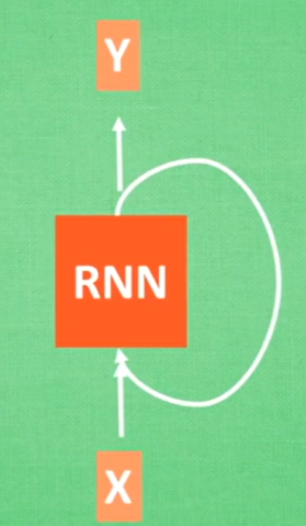
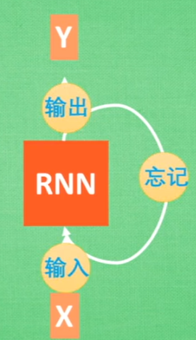
将LSTM内部分为主线和分线部分，控制器输入和忘记将分线有效的学习内容加入主线，最后输出。

3.LSTM的应用

1.自动图片标题生成
《显示并告知：一个神经网络标题生成器》，2014
输入一张图片，预测图片内容，再将单词连接成一个完整的句子。

2.文本自动翻译
3.自动手写体生成
4.音乐的生成
5.字母的生成

更多了解参考：《机器学习博士手把手教你入门LSTM》

二、LSTM源码实例

1.入门–天气预测

博文参考：https://www.rs-online.com/designspark/lstm-1-cn
源码：https://github.com/danrustia11/WeatherLSTM

对 台湾宜兰县的每日环境温度 进行lstm训练：

1. 读取csv：（2000天+温度记录）
2. 数据进行中值滤波和高斯滤波
3. 构建LTSM神经网络
4. 划分训练集和测试集
5. 训练集训练
6. 测试集检测
7. 可视化查看结果

keras+sklearn学习参考源码：

#
# 博文参考：https://www.rs-online.com/designspark/lstm-1-cn
# 源码参考：https://github.com/danrustia11/WeatherLSTM
# LSTM weather prediction demo
# Written by: Dan R 2020
#


#
# Core Keras libraries
#
from numpy import array
from sklearn.metrics import r2_score # 拟合优度
from sklearn.metrics import mean_squared_error  # 均方差
from sklearn.preprocessing import MinMaxScaler
import pandas as pd
import matplotlib.pyplot as plt
import tensorflow as tf  # 随机数生成器，结果可重现
from keras.models import Sequential
from keras.layers import Dense
from keras.layers import LSTM  # LSTM
from keras.layers import Bidirectional  # 双向

#
# For data conditioning
#
from scipy.ndimage import gaussian_filter1d  # 数据调节
from scipy.signal import medfilt

#
# Make results reproducible
#
from numpy.random import seed
seed(1)

tf.random.set_seed(1)
#
# Other essential libraries
#

# Make our plot a bit formal
font = {'family': 'Arial',
        'weight': 'normal',
        'size': 10}
plt.rc('font', **font)


#
# Set input number of timestamps and training days
#
n_timestamp = 10  # 时间戳
train_days = 1500  # number of days to train from 开始的天数
testing_days = 500  # number of days to be predicted 可以预测的天数
n_epochs = 25  # 训练轮数
filter_on = 1  # 激活数据过滤器


#
# Select model type 选择型号类型
# 1: Single cell 单格
# 2: Stacked 堆叠
# 3: Bidirectional 双向
#
model_type = 2

#-----------------------------------------
# 数据集
#-----------------------------------------
# 台湾环境保护局提供的台湾宜兰县的每日环境温度
# url  =  'https://raw.githubusercontent.com/danrustia11/WeatherLSTM/master/data/weather_temperature_yilan.csv'
url = "D:/myworkspace/dataset/WeatherLSTM-master/data/weather_temperature_yilan.csv"
dataset = pd.read_csv(url)
if filter_on == 1:  # 数据集过滤
    dataset['Temperature'] = medfilt(dataset['Temperature'], 3)  # 中值过滤
    dataset['Temperature'] = gaussian_filter1d(
        dataset['Temperature'], 1.2)  # 高斯过滤


#
# Set number of training and testing data 设置训练和测试数据集
#
train_set = dataset[0:train_days].reset_index(drop=True)
test_set = dataset[train_days: train_days+testing_days].reset_index(drop=True)
training_set = train_set.iloc[:, 1:2].values
testing_set = test_set.iloc[:, 1:2].values
#-----------------------------------------
# 数据集完
#-----------------------------------------


#
# Normalize data first
#
sc = MinMaxScaler(feature_range=(0, 1))  # 将数据标准化，范围是0到1
training_set_scaled = sc.fit_transform(training_set)
testing_set_scaled = sc.fit_transform(testing_set)

#
# Split data into n_timestamp
#
def data_split(sequence, n_timestamp):
    X = []
    y = []
    for i in range(len(sequence)):
        end_ix = i + n_timestamp
        if end_ix > len(sequence)-1:
            break
        # i to end_ix as input
        # end_ix as target output
        seq_x, seq_y = sequence[i:end_ix], sequence[end_ix]
        X.append(seq_x)
        y.append(seq_y)
    return array(X), array(y)


X_train, y_train = data_split(training_set_scaled, n_timestamp)
X_train = X_train.reshape(X_train.shape[0], X_train.shape[1], 1)
X_test, y_test = data_split(testing_set_scaled, n_timestamp)
X_test = X_test.reshape(X_test.shape[0], X_test.shape[1], 1)


# 使用Keras建构LSTM模型
if model_type == 1:
    # Single cell LSTM
    model = Sequential()
    model.add(LSTM(units=50, activation='relu',
                   input_shape=(X_train.shape[1], 1)))
    model.add(Dense(units=1))
if model_type == 2:
    # Stacked LSTM
    model = Sequential()
    model.add(LSTM(50, activation='relu', return_sequences=True,
                   input_shape=(X_train.shape[1], 1)))
    model.add(LSTM(50, activation='relu'))
    model.add(Dense(1))
if model_type == 3:
    # Bidirectional LSTM
    model = Sequential()
    model.add(Bidirectional(LSTM(50, activation='relu'),
                            input_shape=(X_train.shape[1], 1)))
    model.add(Dense(1))


#
# Start training 模型训练，batch_size越大越精准，训练消耗越大
#
model.compile(optimizer='adam', loss='mean_squared_error')
history = model.fit(X_train, y_train, epochs=n_epochs, batch_size=32)
loss = history.history['loss']
epochs = range(len(loss))


#
# Get predicted data 测试集预测
#
y_predicted = model.predict(X_test)

#
# 'De-normalize' the data 正规化将数据还原
#
y_predicted_descaled = sc.inverse_transform(y_predicted)
y_train_descaled = sc.inverse_transform(y_train)
y_test_descaled = sc.inverse_transform(y_test)
y_pred = y_predicted.ravel()
y_pred = [round(yx, 2) for yx in y_pred]
y_tested = y_test.ravel()


#
# Show results 显示预测结果，包括原始数据、n个预测天数和前75天
#
plt.figure(figsize=(8, 7))

plt.subplot(3, 1, 1)
plt.plot(dataset['Temperature'], color='black',
         linewidth=1, label='True value')
plt.ylabel("Temperature")
plt.xlabel("Day")
plt.title("All data")


plt.subplot(3, 2, 3)
plt.plot(y_test_descaled, color='black', linewidth=1, label='True value')
plt.plot(y_predicted_descaled, color='red',  linewidth=1, label='Predicted')
plt.legend(frameon=False)
plt.ylabel("Temperature")
plt.xlabel("Day")
plt.title("Predicted data (n days)")

plt.subplot(3, 2, 4)
plt.plot(y_test_descaled[0:75], color='black', linewidth=1, label='True value')
plt.plot(y_predicted_descaled[0:75], color='red', label='Predicted')
plt.legend(frameon=False)
plt.ylabel("Temperature")
plt.xlabel("Day")
plt.title("Predicted data (first 75 days)")

plt.subplot(3, 3, 7)
plt.plot(epochs, loss, color='black')
plt.ylabel("Loss (MSE)")
plt.xlabel("Epoch")
plt.title("Training curve")

plt.subplot(3, 3, 8)
plt.plot(y_test_descaled-y_predicted_descaled, color='black')
plt.ylabel("Residual")
plt.xlabel("Day")
plt.title("Residual plot")

plt.subplot(3, 3, 9)
plt.scatter(y_predicted_descaled, y_test_descaled, s=2, color='black')
plt.ylabel("Y true")
plt.xlabel("Y predicted")
plt.title("Scatter plot")

plt.subplots_adjust(hspace=0.5, wspace=0.3)
plt.show()


mse = mean_squared_error(y_test_descaled, y_predicted_descaled) # 均方误差
r2 = r2_score(y_test_descaled, y_predicted_descaled) # 决定系数（拟合优度）接近1越好
print("mse=" + str(round(mse, 2)))
print("r2=" + str(round(r2, 2)))

2.结果

图一：全部数据（x轴：2000+天数，y轴：温度）
图二：n天温度预测结果
图三：前70天预测结果，可以看见LSTM在不断学习优化
图4，5，6：训练评价因素可视化

3.评价标准

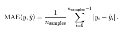
mse均方差（mean-squared-error）

R2 决定系数（拟合优度）

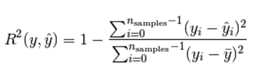
模型越好：r2→1

模型越差：r2→0

更多评价标准参考：学习笔记2：scikit-learn中使用r2_score评价回归模型

同理，在载入自己的数据集时，修改数据集读取模块即可。