转战Pytorch（1）——清点装备

前言

本文适用于曾经使用过Keras,tensorflow，并具备一定深度学习概念的人。由于tensorflow正在完成2.0的转型，越来越多的研究转向Pytorch，因此有必要快速入门一下Pytorch。相比较0基础的人，有一定深度学习基础的同学能够快速的将pytorch和Keras等其他深度学习框架概念相对应，更快的学习pytorch，并将自己的研究迁移到pytorch上来。本文就是完成此目的的第一篇。

当你想要做一件事时，你需要知道有哪些东西你能够使用，有哪些东西需要你自己创造，又要遵守什么样的规则。我们在别的框架里的东西，在pytorch中都有么？都长什么样子？如何使用？本文即将介绍。

1. 基本操作单元

如同其他深度学习框架一样，pytorch也是以张量作为基本操作单元，具体的在代码里，以torch.tensor的形式出现，它与numpy的array基本可以互换。

b = a.numpy()  # a是tensor,b是array
b = torch.from_numpy(a)  # a是array,b是numpy

因此张量具有的运算，它也有，和numpy基本上差不多。不过这里要提及一下一些张量的变换，因为在编程中我们经常需要用到。这里只举几个常用的例子，如拼接、分拆，维度变换以及压缩与反压缩，并将其进行比较差异：

1.1 张量的拼接（torch.cat与torch.stack）

方法1(torch.cat(tensors, dim=0, out=None) → Tensor)

>>> x
tensor([[ 0.6580, -1.0969, -0.4614],
        [-0.1034, -0.5790,  0.1497]])
>>> torch.cat((x, x, x), 0)
tensor([[ 0.6580, -1.0969, -0.4614],
        [-0.1034, -0.5790,  0.1497],
        [ 0.6580, -1.0969, -0.4614],
        [-0.1034, -0.5790,  0.1497],
        [ 0.6580, -1.0969, -0.4614],
        [-0.1034, -0.5790,  0.1497]])
>>> torch.cat((x, x, x), 1)
tensor([[ 0.6580, -1.0969, -0.4614,  0.6580, -1.0969, -0.4614,  0.6580,
         -1.0969, -0.4614],
        [-0.1034, -0.5790,  0.1497, -0.1034, -0.5790,  0.1497, -0.1034,
         -0.5790,  0.1497]])

方法2torch.stack(tensors, dim=0, out=None) → Tensor

>>> x=torch.tensor([[1,2,3],[4,5,6],[7,8,9]])
>>> torch.stack((x,x,x),dim=0)
tensor([[[1, 2, 3],
         [4, 5, 6],
         [7, 8, 9]],
        [[1, 2, 3],
         [4, 5, 6],
         [7, 8, 9]],
        [[1, 2, 3],
         [4, 5, 6],
         [7, 8, 9]]])
>>> y=torch.stack((x,x,x),dim=1)
tensor([[[1, 2, 3],
         [1, 2, 3],
         [1, 2, 3]],
        [[4, 5, 6],
         [4, 5, 6],
         [4, 5, 6]],
        [[7, 8, 9],
         [7, 8, 9],
         [7, 8, 9]]])

其实能看到cat是按照指定维度进行拼接，而stack则仍然将每个组成部分看做是独立的个体，在拼接的时候，额外增加出一个维度出来。

1.2 张量的分拆（torch.chunk与torch.split）

方法1torch.chunk(input, chunks, dim=0) → List of Tensors
chunk可以指定维度进行拆解

>>> torch.chunk(y,3,dim=0)
(tensor([[[1, 2, 3],
         [1, 2, 3],
         [1, 2, 3]]]), 
 tensor([[[4, 5, 6],
         [4, 5, 6],
         [4, 5, 6]]]), 
 tensor([[[7, 8, 9],
         [7, 8, 9],
         [7, 8, 9]]]))
>>> torch.chunk(y,2,dim=0)
(tensor([[[1, 2, 3],
         [1, 2, 3],
         [1, 2, 3]],
        [[4, 5, 6],
         [4, 5, 6],
         [4, 5, 6]]]), 
tensor([[[7, 8, 9],
         [7, 8, 9],
         [7, 8, 9]]]))

方法2torch.split(tensor, split_size_or_sections, dim=0)
与split相同，不过其第二个维度可以是一个列表，表示如何进行切分。例如，split_size_or_sections=1，则表示每个部分只有1个元素，如果是split_size_or_sections=（1,2）,则表示第一个部分的大小为1，第二个部分大小为2。

>>> torch.split(y,1,dim=0)
(tensor([[[1, 2, 3],
         [1, 2, 3],
         [1, 2, 3]]]), 
 tensor([[[4, 5, 6],
         [4, 5, 6],
         [4, 5, 6]]]),
 tensor([[[7, 8, 9],
         [7, 8, 9],
         [7, 8, 9]]]))
>>> torch.split(y,(1,2),dim=0)
(tensor([[[1, 2, 3],
         [1, 2, 3],
         [1, 2, 3]]]), 
 tensor([[[4, 5, 6],
         [4, 5, 6],
         [4, 5, 6]],
        [[7, 8, 9],
         [7, 8, 9],
         [7, 8, 9]]]))

1.3 张量的维度变换（torch.Tensor.view和torch.reshape）

方法1torch.Tensor.view(*shape) → Tensor
view可以用来将张量的形状的改变。

>>> x = torch.randn(4, 4)
>>> x.size()
torch.Size([4, 4])
>>> y = x.view(16)
>>> y.size()
torch.Size([16])
>>> z = x.view(-1, 8)  # the size -1 is inferred from other dimensions
>>> z.size()
torch.Size([2, 8])

>>> a = torch.randn(1, 2, 3, 4)
>>> a.size()
torch.Size([1, 2, 3, 4])
>>> b = a.transpose(1, 2)  # Swaps 2nd and 3rd dimension
>>> b.size()
torch.Size([1, 3, 2, 4])
>>> c = a.view(1, 3, 2, 4)  # Does not change tensor layout in memory
>>> c.size()
torch.Size([1, 3, 2, 4])
>>> torch.equal(b, c)
False

方法2torch.reshape(input, shape) → Tensor

>>> a = torch.arange(4.)
>>> torch.reshape(a, (2, 2))
tensor([[ 0.,  1.],
        [ 2.,  3.]])
>>> b = torch.tensor([[0, 1], [2, 3]])
>>> torch.reshape(b, (-1,))
tensor([ 0,  1,  2,  3])

另一个和这个一样的操作是torch.Tensor.reshape(*shape) → Tensor

reshape与view的区别是reshape不依赖于内存中数据的连续性,view前后的tensor指向的同一数据区，view函数只能由于contiguous的张量上，具体而言，就是在内存中连续存储的张量。所以，当tensor之前调用了transpose, permute函数就会是tensor内存中变得不再连续，就不能调用view函数。

1.4 张量的压缩和反压缩（torch.squeeze和torch.unsqueeze）

压缩torch.squeeze(input, dim=None, out=None) → Tensor
当我们需要去除一个维度只有上只有一个样例的时候，压缩是一个好的操作。

>>> x = torch.zeros(2, 1, 2, 1, 2)
>>> x.size()
torch.Size([2, 1, 2, 1, 2])
>>> y = torch.squeeze(x)  # 不指定维度，所有维度都检查
>>> y.size()
torch.Size([2, 2, 2])
>>> y = torch.squeeze(x, 0) # 第0维度不是1，因此不操作。
>>> y.size()
torch.Size([2, 1, 2, 1, 2])
>>> y = torch.squeeze(x, 1) # 第1维度是1，因此删除该维度。
>>> y.size()
torch.Size([2, 2, 1, 2])

反压缩torch.unsqueeze(input, dim, out=None) → Tensor
有时候我们需要对一个样例增加一个batch的维度，从而输入到模型中，这时候unsequeeze操作就比较有用了。

>>> x = torch.tensor([1, 2, 3, 4])
>>> torch.unsqueeze(x, 0)
tensor([[ 1,  2,  3,  4]])  # 1*4
>>> torch.unsqueeze(x, 1)
tensor([[ 1],[ 2],[ 3],[ 4]])  #4*1

2. 基本模型（网络）

这里我们主要介绍基本网络以及常见的一些层。

2.1 基本模型（torch.nn.Module）

所有的模型都需要继承此类，然后才能完成网络配置、前向传播过程等。

import torch.nn as nn
import torch.nn.functional as F

class Model(nn.Module):
    def __init__(self):
        super(Model, self).__init__()
        # 这里构建我们自己的模型，这些组成模型的层将会在下面的前向传播中使用。
        self.conv1 = nn.Conv2d(1, 20, 5)
        self.conv2 = nn.Conv2d(20, 20, 5)

    def forward(self, x):
    # 这里写整个向量的流转过程，此时X就是一个实例，你可以对它进行任何的操作。
        x = F.relu(self.conv1(x))
        return F.relu(self.conv2(x))

看到这里你是不是要惊呼，TF2.0和pytorch实在长的太像了，没错，这也是大势所趋，将来必定一统天下。
当然，如果你的模型比较简单，是一个序贯模型的话，pytorch里提供和keras一样的基础模型Sequential

# Example of using Sequential
model = nn.Sequential(
          nn.Conv2d(1,20,5),
          nn.ReLU(),
          nn.Conv2d(20,64,5),
          nn.ReLU()
        )

# Example of using Sequential with OrderedDict
model = nn.Sequential(OrderedDict([
          ('conv1', nn.Conv2d(1,20,5)),
          ('relu1', nn.ReLU()),
          ('conv2', nn.Conv2d(20,64,5)),
          ('relu2', nn.ReLU())
        ]))

2.2 卷积神经网络

这里我们只介绍常用的两种卷积1维卷积和2维卷积

2.2.1 一维卷积

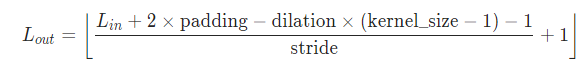
一维卷积torch.nn.Conv1d(in_channels, out_channels, kernel_size, stride=1, padding=0, dilation=1, groups=1, bias=True, padding_mode='zeros')

可以看到这里的 $C_{in}$=in_channels, $C_{out}$=out_channels, $L_out$是算出来的。

下面是一个简单的实例，让我们明白发生了什么。

>>> import torch.nn as nn
>>> m=nn.Conv1d(16,33,3,stride=2)
>>> input=torch.randn(20,16,50)
>>> output=m(input)
>>> output.size()
torch.Size([20, 33, 24])

如果你对于具体的卷积过程还不够了解，建议看《卷积的图示》

2.2.2 二维卷积

二维卷积torch.nn.Conv2d(in_channels, out_channels, kernel_size, stride=1, padding=0, dilation=1, groups=1, bias=True, padding_mode='zeros')

二维卷积则是在一个二维的张量上进行卷积。其操作基本一致：

# With square kernels and equal stride
>>> m = nn.Conv2d(16, 33, 3, stride=2)
>>> # non-square kernels and unequal stride and with padding
>>> m = nn.Conv2d(16, 33, (3, 5), stride=(2, 1), padding=(4, 2))
>>> # non-square kernels and unequal stride and with padding and dilation
>>> m = nn.Conv2d(16, 33, (3, 5), stride=(2, 1), padding=(4, 2), dilation=(3, 1))
>>> input = torch.randn(20, 16, 50, 100)
>>> output = m(input)

2.3 循环神经网络

另一个常用的就是循环神经网络，主要使用的有RNN,GRU和LSTM，我们来看一下pytorch的表现形式是如何的。

2.3.1 RNN

RNNtorch.nn.RNN(*args, **kwargs)
作为基础的循环神经网络，它的局部结构比较简单，公式如下（记住在论文里，公式真的很重要）。

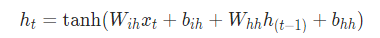
这里的tanh可以换成relu，要用到参数。其形象化为：

下面我们看看参数都有哪些可以用的，我们这里挑几个需要注意的：
参数
input_size– The number of expected features in the input x
hidden_size– The number of features in the hidden state h
num_layers– Number of recurrent layers. 这一个非常好的参数，当num_layers>1时，就是stack-RNN的形式。
nonlinearity– 可选择 ‘tanh’ or ‘relu’. Default: ‘tanh’
batch_first– 默认为: False。RNN的输入是(seq_len, batch_size, input_size)，batch_size位于第二维度！虽然你可以将batch_size和序列长度seq_len对换位置，此时只需要令batch_first=True。
但是为什么RNN输入默认不是batch first=True？这是为了便于并行计算。因为cuDNN中RNN的API就是batch_size在第二维度！（pytorch的batch_first）。
dropout– 丢弃值0-1，0为不丢弃，1为完全丢弃。
bidirectional– 是否是双向，默认为 False。

从这可以看出pytorch给出的可变化性还是挺多的，基本满足使用，更好的是要看输入和输出：
输入：input, h_0
这里input是我们的输入,其形状为 (seq_len, batch, input_size)，而且不用担心的是，我们可以使用torch.nn.utils.rnn.pack_padded_sequence() 格式化输入。h_0为初始化隐藏向量，比如我们可以接一个之前的外来因素进行初始化。

输出：output, h_n
output为输出向量，其形状为(seq_len, batch, num_directions * hidden_size)。h_n为结束向量，可以当做另一个的初始化向量。

例子

>>> rnn = nn.RNN(10, 20, 2)
>>> input = torch.randn(5, 3, 10)
>>> h0 = torch.randn(2, 3, 20)
>>> output, hn = rnn(input, h0)

2.3.2 GRU

GRUtorch.nn.GRU(*args, **kwargs)
GRU比普通的RNN要复杂一些，主要是它增加了门控机制，其公式如下：

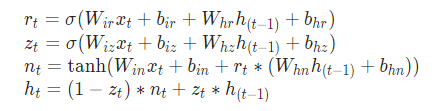
其形象化为：

其参数、输入和输出都和普通的RNN一样，没有什么区别。
下面是一个例子：

>>> rnn = nn.GRU(10, 20, 2)
>>> input = torch.randn(5, 3, 10)
>>> h0 = torch.randn(2, 3, 20)
>>> output, hn = rnn(input, h0)

2.3.2 LSTM

LSTMtorch.nn.LSTM(*args, **kwargs)相比较RNN和GRU，更加复杂一些，因为它能够拥有长的短时记忆，由于它多了一个细胞状态（C），其形式化表达如下。

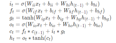
其形象化表达如下：

由于多出了一个细胞状态（也就是图中加粗的部分），因此其输入和输出也分别多了一个参数。
输入: input, (h_0, c_0)
h_0和c_0的形状相同，都是(num_layers * num_directions, batch, hidden_size)。
输出: output, (h_n, c_n)
输出和输入都一样。

下面这是一个使用的例子。

>>> rnn = nn.LSTM(10, 20, 2)
>>> input = torch.randn(5, 3, 10)
>>> h0 = torch.randn(2, 3, 20)
>>> c0 = torch.randn(2, 3, 20)
>>> output, (hn, cn) = rnn(input, (h0, c0))

3. 线性层

线性层是最基础的层，主要就是进行一些线性变换，其中像多层感知机就是由此部分组成的。这里我们介绍两个常用的层，线性层和双线性层。

3.1 线性层

线性层torch.nn.Linear(in_features, out_features, bias=True)主要进行一个线性变换，使得抽取一些特征并改变其维度。公式如下：

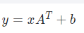
输入输出如下：
Input:(N,*,in_features)
Output:(N,*,out_features)
这就是说，输入输出只关心最后一个维度是否匹配就可以了，前面的维度不用考虑。

例子如下：

>>> m = nn.Linear(20, 30)
>>> input = torch.randn(128, 20)
>>> output = m(input)
>>> print(output.size())
torch.Size([128, 30])

3.2 双线性层

双线性层torch.nn.Bilinear(in1_features, in2_features, out_features, bias=True)相比较线性层，增加了一个输入，这也使得它可以用来进行两个输入的向量匹配等操作。其公式如下：

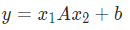
例子如下：

>>> m = nn.Bilinear(20, 30, 40)
>>> input1 = torch.randn(128, 20)
>>> input2 = torch.randn(128, 30)
>>> output = m(input1, input2)
>>> print(output.size())
torch.Size([128, 40])

4. 非线性激活层

只使用线性层的神经网络在上个世纪60年代就已经被否定了，因此，需要使用非线性的激活函数来增强神经网络的表达能力。这里我们也只介绍一些常见的非线性激活层。

4.1 Relu

Relutorch.nn.ReLU(inplace=False)是一个比较常用的非线性激活函数，其形式化表达如下：
$ReLU(x)=max(0,x)$

该网络层并没有进行任何维度的变换，只是将输入映射到输出中。

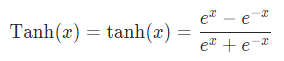
4.2 Tanh

Tanhtorch.nn.Tanh是另一个常用的激活函数，其形式比较简单，也没有参数：

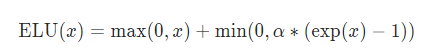
4.3 ELU

ELUtorch.nn.ELU(alpha=1.0, inplace=False)则是最近比较喜欢用的一个激活函数，解决Relu负数时是0的问题。

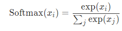
4.4 Softmax

Softmaxtorch.nn.Softmax(dim=None)和其他几个激活函数不同，它一般被用来作为模型分类的最后一层，用于概率归一化。

但是，在pytorch里，这个也不怎么常用了，一般都使用logsoftmaxtorch.nn.LogSoftmax(dim=None)和NLLLtorch.nn.NLLLoss(weight=None, size_average=None, ignore_index=-100, reduce=None, reduction='mean')损失函数搭配使用，不然的话，只需要使用交叉熵损失函数torch.nn.CrossEntropyLoss(weight=None, size_average=None, ignore_index=-100, reduce=None, reduction='mean')即可。

5. 损失函数

就像刚才讲的那样，我们在计算反向传播时，需要损失函数，上面提到了2个损失函数，我们这里就详细介绍一些这几个。

5.1 NLLL

NLLLtorch.nn.NLLLoss(weight=None, size_average=None, ignore_index=-100, reduce=None, reduction='mean')损失函数一般搭配logsoftmax一起使用，也就是极大似然估计。更多详情可见《损失函数具体在做什么》。

这里需要注意的一个是它的输入输出的大小。
输入：(N,C) N是样本数，C是类别数
输出：(N) 是一个个离散的样本类别。（0~C-1）

例子：

>>> m = nn.LogSoftmax(dim=1)
>>> loss = nn.NLLLoss()
>>> # input is of size N x C = 3 x 5
>>> input = torch.randn(3, 5, requires_grad=True)
>>> # each element in target has to have 0 <= value < C
>>> target = torch.tensor([1, 0, 4])
>>> output = loss(m(input), target)
>>> output.backward()
>>>
>>>
>>> # 2D loss example (used, for example, with image inputs)
>>> N, C = 5, 4
>>> loss = nn.NLLLoss()
>>> # input is of size N x C x height x width
>>> data = torch.randn(N, 16, 10, 10)
>>> conv = nn.Conv2d(16, C, (3, 3))
>>> m = nn.LogSoftmax(dim=1)
>>> # each element in target has to have 0 <= value < C
>>> target = torch.empty(N, 8, 8, dtype=torch.long).random_(0, C)
>>> output = loss(m(conv(data)), target)
>>> output.backward()

5.2 交叉熵损失函数

交叉熵损失函数torch.nn.CrossEntropyLoss(weight=None, size_average=None, ignore_index=-100, reduce=None, reduction='mean')是最常用的一种损失函数，它等价于logsoftmax+NLLL的效果。输入输出大小与NLLL一样，使用上也类似。

例子：

>>> loss = nn.CrossEntropyLoss()
>>> input = torch.randn(3, 5, requires_grad=True)
>>> target = torch.empty(3, dtype=torch.long).random_(5)
>>> output = loss(input, target)
>>> output.backward()

其他损失函数这里就不一一赘述了，更多的可以参见《pytorch损失函数的十八罗汉》。有一个需要注意的是，pytorch可以看到整个模型的任何一个部分，因此可以在模型的任何一部分增加损失函数用于学习。

6. 小结

本文我们简要的梳理了一下pytorch都有哪些可以使用的层及其相关函数，这让我们对于接下来能做的事情做到心里有数，接下来我们就要进入行车快速道了，坐稳了！（transformer也被集成到pytorch中，这对我们是一个好消息）