什么是PyTorch?
PyTorch是一个基于python的科学计算包,主要定位两类人群:
- NumPy的替代品,可以利用GPU的性能进行计算
- 深度学习研究平台拥有足够的灵活性和速度
PyTorch的安装(cpu版)
因为没有安装cuda所以这里我就只安装了CPU版本的,安装参考网站:https://pytorch.org/
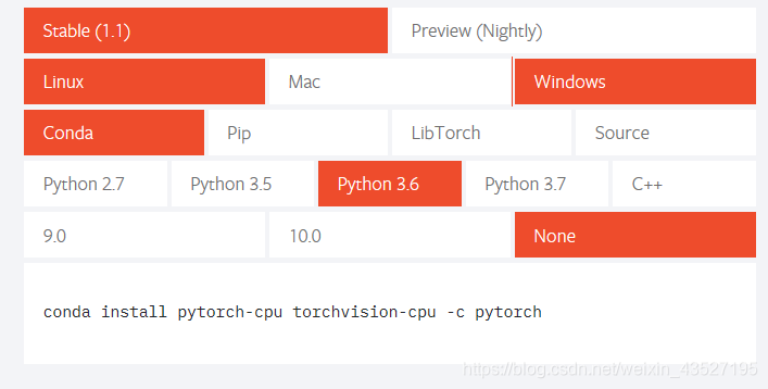
按照图片最下面一行在annoconda命令窗口敲就行,我这里是使用conda进行安装的(速度还很快)
安装完成后:
python
import torch
torch.version
正确显示就代表安装成功了。
PyTorch学习网址
https://shimo.im/docs/CVkTvCwCdw9K3WpD
PyTorch实现神经网络
一个典型的神经网络训练过程包括以下几点:
1. 定义一个包含可训练参数的网络
2. 迭代整个输入
3. 通过神经网络处理输入
4. 计算损失(loss)
5. 反向传播梯度到神经网络的参数
6. 更新网络的参数,典型的用一个简单的更新方法:weight=weight-learning_rate*gradient
神经网络可以通过 torch.nn 包来构建。
现在对于自动梯度(autograd)有一些了解,神经网络是基于自动梯度 (autograd)来定义一些模型。一个 nn.Module 包括层和一个方法 forward(input) 它会返回输出(output)。
代码实现:
import torch
import torch.nn as nn
import torch.nn.functional as F
1)定义神经网络
#定义神经网络
class Net(nn.Module):
    def __init__(self):
        super(Net,self).__init__()
        #建立两个卷积层,self.conv1和self.conv2,注意,这些层都是不含激活函数的
        # 1 input image channel, 6 output channels, 5x5 square convolution(5*5的卷积核)
        # kernel
        self.conv1 = nn.Conv2d(1,6,5)
        self.conv2 = nn.Conv2d(6,16,5)
        #三个全连接层
        # an affine operation: y = Wx + b
        self.fc1 = nn.Linear(16*5*5,120)
        self.fc2 = nn.Linear(120,84)
        self.fc3 = nn.Linear(84,10)

    def forward(self,x):
        #Max pooling over a (2,2) window
        x = F.max_pool2d(F.relu(self.conv1(x)),(2,2))
        # if the size is a square you can only specify a single number
        x = F.max_pool2d(F.relu(self.conv2(x)),2)
        x = x.view(-1,self.num_flat_feature(x))
        x = F.relu(self.fc1(x))
        x = F.relu(self.fc2(x))
        x = self.fc3(x)
        return x

    def num_flat_feature(self,x):
        size = x.size()[1:]#all dimensions except the batch dimension
        num_features = 1
        for s in size:
            num_features *= s
        return num_features

net = Net()
print(net)
Net(
  (conv1): Conv2d(1, 6, kernel_size=(5, 5), stride=(1, 1))
  (conv2): Conv2d(6, 16, kernel_size=(5, 5), stride=(1, 1))
  (fc1): Linear(in_features=400, out_features=120, bias=True)
  (fc2): Linear(in_features=120, out_features=84, bias=True)
  (fc3): Linear(in_features=84, out_features=10, bias=True)
)
2)处理输入,调用反向传播
#一个模型可训练的参数通过net.parameters()返回
params = list(net.parameters())
print(len(params)) #10=5*2(weights*bias)
print(params[0].size()) # conv1's .weight
10
torch.Size([6, 1, 5, 5])
#随机生成一个32*32的输入
input = torch.randn(1,1,32,32)
out = net(input)
print(out)
tensor([[ 0.0773, -0.0392, -0.0182, -0.0400, -0.1043,  0.0837,  0.0295, -0.0494,
          0.1041,  0.0829]], grad_fn=<AddmmBackward>)
#把所有的梯度参数置0,用随机的梯度来反向传播
net.zero_grad()
out.backward(torch.randn(1,10))
3)损失函数
#损失函数
#一个损失函数需要一对输入:模型输出和目标,然后计算一个值来评估输出距离目标有多远。
#有一些不同的损失函数在 nn 包中。一个简单的损失函数就是 nn.MSELoss ,这计算了均方误差。
output = net(input)
target = torch.randn(10) #a dummy target
target = target.view(1,-1) #make it the same shape as output
criterion = nn.MSELoss()
loss = criterion(output,target)
print(loss)
tensor(0.6606, grad_fn=<MseLossBackward>)
现在,如果你跟随损失到反向传播路径,可以使用它的 .grad_fn 属性,你将会看到一个这样的计算图:
input -> conv2d -> relu -> maxpool2d -> conv2d -> relu -> maxpool2d
-> view -> linear -> relu -> linear -> relu -> linear
-> MSELoss
-> loss
print(loss.grad_fn)
print(loss.grad_fn.next_functions[0][0])#Linear
print(loss.grad_fn.next_functions[0][0].next_functions[0][0])#ReLU
<MseLossBackward object at 0x00000229E3CD9EB8>
<AddmmBackward object at 0x00000229E3CD9FD0>
<AccumulateGrad object at 0x00000229E3CD9EB8>
4)反向传播
#反向传播
#为了实现反向传播损失,我们所有需要做的事情仅仅是使用loss.backward()。你需要清空现存梯度
net.zero_grad()  # zeroes the gradient buffers of all parameters
print('conv1.bias.grad before backward')
print(net.conv1.bias.grad)
loss.backward()
print('conv1.bias.grad after backward')
print(net.conv1.bias.grad)
conv1.bias.grad before backward
tensor([0., 0., 0., 0., 0., 0.])
conv1.bias.grad after backward
tensor([ 0.0007, -0.0022, -0.0093,  0.0020,  0.0158, -0.0037])
5)更新网络参数
#更新神经网络参数
#最简单的规则就是weight = weight - learning_rate*gradient
learning_rate = 0.01
for f in net.parameters():
    f.data.sub_(f.grad.data*learning_rate)
尽管如此,如果你是用神经网络,你想使用不同的更新规则,类似于 SGD, Nesterov-SGD, Adam, RMSProp, 等。为了让这可行,我们建立了一个小包:torch.optim 实现了所有的方法。使用它非常的简单。
import torch.optim as optim
# create your optimizer
optimizer = optim.SGD(net.parameters(), lr=0.01)
# in your training loop:
optimizer.zero_grad()   # zero the gradient buffers
output = net(input)
loss = criterion(output, target)
loss.backward()
optimizer.step()    # Does the update
神经网络实现到此结束,对神经网络小白来说,这个代码实现只读了个半懂,加油!!!
下载 Jupyter 源代码:
http://pytorchchina.com/wp-content/uploads/2018/12/neural_networks_tutorial.ipynb_.zip
推荐网址:
https://github.com/fendouai/pytorch1.0-cn
