Caffe: (三) LeNet （训练测试网络，solver的参数理解，python接口搭建网络结构）

from pylab import *
%matplotlib inline

import caffe

import os
caffe_root = "Path to caffe"
os.chdir(caffe_root)

os.getcwd()

“Path to caffe”

!data/mnist/get_mnist.sh

Downloading...

# prepare data
!examples/mnist/create_mnist.sh

Creating lmdb...
I0305 15:36:48.341755 32245 db_lmdb.cpp:35] Opened lmdb examples/mnist/mnist_train_lmdb
I0305 15:36:48.341928 32245 convert_mnist_data.cpp:88] A total of 60000 items.
I0305 15:36:48.341936 32245 convert_mnist_data.cpp:89] Rows: 28 Cols: 28
I0305 15:36:53.402994 32245 convert_mnist_data.cpp:108] Processed 60000 files.
I0305 15:36:53.948365 32384 db_lmdb.cpp:35] Opened lmdb examples/mnist/mnist_test_lmdb
I0305 15:36:53.948536 32384 convert_mnist_data.cpp:88] A total of 10000 items.
I0305 15:36:53.948545 32384 convert_mnist_data.cpp:89] Rows: 28 Cols: 28
I0305 15:36:54.727614 32384 convert_mnist_data.cpp:108] Processed 10000 files.
Done.

from caffe import layers as L, params as P
def lenet(lmdb, batch_size):
    # our version of LeNet: a series of linear and simple nonlinear transformations
    n = caffe.NetSpec()
    n.data, n.label = L.Data(batch_size=batch_size, backend=P.Data.LMDB, 
                             source=lmdb, transform_param=dict(scale=1./255),
                             ntop=2)

    n.conv1 = L.Convolution(n.data, kernel_size =5, num_output=20,
                           weight_filler=dict(type='xavier'))
    n.pool1 = L.Pooling(n.conv1, kernel_size=2, stride=2, pool=P.Pooling.MAX)
    n.conv2 = L.Convolution(n.pool1, kernel_size=5, num_output=50, 
                           weight_filler=dict(type='xavier'))
    n.pool2 = L.Pooling(n.conv2, kernel_size=2, stride=2, pool=P.Pooling.MAX)
    n.fc1 = L.InnerProduct(n.pool2, num_output=500, weight_filler=dict(type='xavier'))
    n.relu1 = L.ReLU(n.fc1, in_place=True)
    n.score = L.InnerProduct(n.relu1, num_output=10, weight_filler=dict(type='xavier'))
    n.loss = L.SoftmaxWithLoss(n.score, n.label)
    return n.to_proto()

os.chdir(caffe_root+"/examples")

os.getcwd()

'path to caffe/examples'

os.listdir()

['CMakeLists.txt',
 'pycaffe',
 'imagenet',
 '00-classification.ipynb',
 'mnist',
 '01-learning-lenet.ipynb',
 'net_surgery',
 'cifar10',
 'web_demo',
 'siamese',
 'hdf5_classification',
 'feature_extraction',
 'finetune_pascal_detection',
 'net_surgery.ipynb',
 'cpp_classification',
 'detection.ipynb',
 'finetune_flickr_style',
 'brewing-logreg.ipynb',
 'images',
 'pascal-multilabel-with-datalayer.ipynb',
 '02-fine-tuning.ipynb']

with open('mnist/lenet_auto_train.prototxt', 'w') as f:
    f.write(str(lenet('mnist/mnist_train_lmdb', 64)))

with open('mnist/lenet_auto_test.prototxt', 'w') as f:
    f.write(str(lenet('mnist/mnist_test_lmdb', 100)))

!cat mnist/lenet_auto_train.prototxt

layer {
  name: "data"
  type: "Data"
  top: "data"
  top: "label"
  transform_param {
    scale: 0.003921568859368563
  }
  data_param {
    source: "mnist/mnist_train_lmdb"
    batch_size: 64
    backend: LMDB
  }
}
layer {
  name: "conv1"
  type: "Convolution"
  bottom: "data"
  top: "conv1"
  convolution_param {
    num_output: 20
    kernel_size: 5
    weight_filler {
      type: "xavier"
    }
  }
}
layer {
  name: "pool1"
  type: "Pooling"
  bottom: "conv1"
  top: "pool1"
  pooling_param {
    pool: MAX
    kernel_size: 2
    stride: 2
  }
}
layer {
  name: "conv2"
  type: "Convolution"
  bottom: "pool1"
  top: "conv2"
  convolution_param {
    num_output: 50
    kernel_size: 5
    weight_filler {
      type: "xavier"
    }
  }
}
layer {
  name: "pool2"
  type: "Pooling"
  bottom: "conv2"
  top: "pool2"
  pooling_param {
    pool: MAX
    kernel_size: 2
    stride: 2
  }
}
layer {
  name: "fc1"
  type: "InnerProduct"
  bottom: "pool2"
  top: "fc1"
  inner_product_param {
    num_output: 500
    weight_filler {
      type: "xavier"
    }
  }
}
layer {
  name: "relu1"
  type: "ReLU"
  bottom: "fc1"
  top: "fc1"
}
layer {
  name: "score"
  type: "InnerProduct"
  bottom: "fc1"
  top: "score"
  inner_product_param {
    num_output: 10
    weight_filler {
      type: "xavier"
    }
  }
}
layer {
  name: "loss"
  type: "SoftmaxWithLoss"
  bottom: "score"
  bottom: "label"
  top: "loss"
}

!cat mnist/lenet_auto_solver.prototxt

# The train/test net protocol buffer definition
train_net: "mnist/lenet_auto_train.prototxt"
test_net: "mnist/lenet_auto_test.prototxt"
# test_iter specifies how many forward passes the test should carry out.
# In the case of MNIST, we have test batch size 100 and 100 test iterations,
# covering the full 10,000 testing images.
test_iter: 100
# Carry out testing every 500 training iterations.
test_interval: 500
# The base learning rate, momentum and the weight decay of the network.
base_lr: 0.01
momentum: 0.9
weight_decay: 0.0005
# The learning rate policy
lr_policy: "inv"
gamma: 0.0001
power: 0.75
# Display every 100 iterations
display: 100
# The maximum number of iterations
max_iter: 10000
# snapshot intermediate results
snapshot: 5000
snapshot_prefix: "mnist/lenet"

caffe.set_device(0)
caffe.set_mode_gpu()

# load the solver and create train and test nets
solver = None # ignore this workaround for lmdb data(can't instantiate two solvers on the same data)
solver = caffe.SGDSolver('mnist/lenet_auto_solver.prototxt')

# each output is (batch_size, feature dim, spatial dim)
[(k, v.data.shape) for k, v in solver.net.blobs.items()]

[('data', (64, 1, 28, 28)),
 ('label', (64,)),
 ('conv1', (64, 20, 24, 24)),
 ('pool1', (64, 20, 12, 12)),
 ('conv2', (64, 50, 8, 8)),
 ('pool2', (64, 50, 4, 4)),
 ('fc1', (64, 500)),
 ('score', (64, 10)),
 ('loss', ())]

# just print the weight size 
[(k, v[0].data.shape, v[1].data.shape) for k, v in solver.net.params.items()]

[('conv1', (20, 1, 5, 5), (20,)),
 ('conv2', (50, 20, 5, 5), (50,)),
 ('fc1', (500, 800), (500,)),
 ('score', (10, 500), (10,))]

solver.net.forward() #train net

{'loss': array(2.3818157, dtype=float32)}

solver.test_nets[0].forward()

{'loss': array(2.3772972, dtype=float32)}

# we use a little tricks to tile the first eight images
imshow(solver.net.blobs['data'].data[:8, 0].transpose(1,0,2).reshape(28, 8*28), 
      cmap='gray')
axis('off')
print('train labels: ', solver.net.blobs['label'].data[:8])

train labels:  [5. 0. 4. 1. 9. 2. 1. 3.]

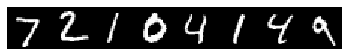
# we use a little tricks to tile the first eight images
imshow(solver.test_nets[0].blobs['data'].data[:8, 0].transpose(1,0,2).reshape(28, 8*28), 
      cmap='gray')
axis('off')
print('test labels: ', solver.test_nets[0].blobs['label'].data[:8])

test labels:  [7. 2. 1. 0. 4. 1. 4. 9.]

solver.step(1)

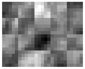
imshow(solver.net.params['conv1'][0].diff[:,0].reshape(4, 5, 5, 5)
      .transpose(0,2,1,3).reshape(4*5, 5*5), cmap='gray')
axis('off')

(-0.5, 24.5, 19.5, -0.5)

%%time
niter = 200
test_interval = 25
# losses will also be stored in the log
train_loss = zeros(niter)
test_acc = zeros(int(np.ceil(niter/test_interval)))
output = zeros((niter, 8, 10))

# the main solver loop
for it in range(niter):
    solver.step(1) # SGD by Caffe
    # store the train loss
    train_loss[it] = solver.net.blobs['loss'].data
    
    # store the output on the first test batch
    # start the forward pass at conv1 to avoid loading new data
    solver.test_nets[0].forward(start='conv1')
    output[it] = solver.test_nets[0].blobs['score'].data[:8]
    
    # run a full test every so often
    # (Caffe can also do this for us and write to a log, but we show here
    # how to do it directly in python, where moe complicated things are easier.)
    if it % test_interval == 0:
        print('Iteration', it, 'testing ...')
        correct = 0
        for test_it in range(100):
            solver.test_nets[0].forward()
            correct += sum(solver.test_nets[0].blobs['score'].data.argmax(1)
                          == solver.test_nets[0].blobs['label'].data)
        test_acc[it//test_interval]=correct/1e4

Iteration 0 testing ...
Iteration 25 testing ...
Iteration 50 testing ...
Iteration 75 testing ...
Iteration 100 testing ...
Iteration 125 testing ...
Iteration 150 testing ...
Iteration 175 testing ...
CPU times: user 1.85 s, sys: 404 ms, total: 2.26 s
Wall time: 1.83 s

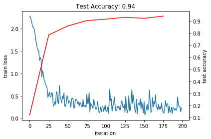
_, ax1 = subplots()
ax2 = ax1.twinx()
ax1.plot(arange(niter), train_loss)
ax2.plot(test_interval*arange(len(test_acc)), test_acc, 'r')
ax1.set_xlabel('iteration')
ax1.set_ylabel('train loss')
ax2.set_ylabel('test accuracy')
ax2.set_title('Test Accuracy: {:.2f}'.format(test_acc[-1]))

Text(0.5, 1.0, 'Test Accuracy: 0.94')

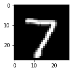
for i in range(8):
    figure(figsize=(2, 2))
    imshow(solver.test_nets[0].blobs['data'].data[i,0],cmap='gray')
    figure(figsize=(10, 2))
    imshow(output[:50, i].T, interpolation='nearest',cmap='gray')
    xlabel('iteration')
    ylabel('label')

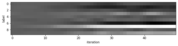
这里可以输出八对，就不输出了，太多了/(ㄒoㄒ)/~~

for i in range(8):
    figure(figsize=(2, 2))
    imshow(solver.test_nets[0].blobs['data'].data[i,0], cmap='gray')
    figure(figsize=(10,2))
    imshow(exp(output[:50, i].T)/exp(output[:50, i].T).sum(0), 
           interpolation='nearest', cmap='gray')
    xlabel('iteration')
    ylabel('label')

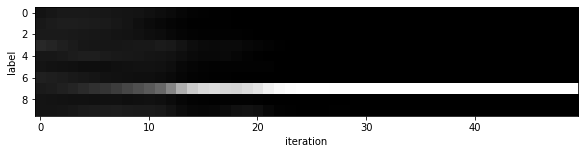
这里也是，节省点篇幅。。。

train_net_path ='mnist/custom_auto_train.prototxt'
test_net_path = 'mnist/custom_auto_test.prototxt'
solver_config_path = 'mnist/custom_auto_solver.prototxt'

# define net
def custom_net(lmdb, batch_size):
    # define your own net!
    n = caffe.NetSpec()
    
    # keep this data layer for all networks
    n.data, n.label = L.Data(batch_size=batch_size, backend=P.Data.LMDB, source=lmdb,
                             transform_param=dict(scale=1./255), ntop=2)
    
    # EDIT HERE to try different networks
    # this single layer defines a simple linear classifier
    # (in particular this defines a multiway logistic regression)
    n.score =   L.InnerProduct(n.data, num_output=10, weight_filler=dict(type='xavier'))
    
    # EDIT HERE this is the LeNet variant we have already tried
    # n.conv1 = L.Convolution(n.data, kernel_size=5, num_output=20, weight_filler=dict(type='xavier'))
    # n.pool1 = L.Pooling(n.conv1, kernel_size=2, stride=2, pool=P.Pooling.MAX)
    # n.conv2 = L.Convolution(n.pool1, kernel_size=5, num_output=50, weight_filler=dict(type='xavier'))
    # n.pool2 = L.Pooling(n.conv2, kernel_size=2, stride=2, pool=P.Pooling.MAX)
    # n.fc1 =   L.InnerProduct(n.pool2, num_output=500, weight_filler=dict(type='xavier'))
    # EDIT HERE consider L.ELU or L.Sigmoid for the nonlinearity
    # n.relu1 = L.ReLU(n.fc1, in_place=True)
    # n.score =   L.InnerProduct(n.fc1, num_output=10, weight_filler=dict(type='xavier'))
    
    # keep this loss layer for all networks
    n.loss =  L.SoftmaxWithLoss(n.score, n.label)
    
    return n.to_proto()
    

with open(train_net_path, 'w') as f:
    f.write(str(custom_net('mnist/mnist_train_lmdb', 64)))    
with open(test_net_path, 'w') as f:
    f.write(str(custom_net('mnist/mnist_test_lmdb', 100)))

# define solver
### define solver
from caffe.proto import caffe_pb2
s = caffe_pb2.SolverParameter()

# Set a seed for reproducible experiments:
# this controls for randomization in training.
s.random_seed = 0xCAFFE

# Specify locations of the train and (maybe) test networks.
s.train_net = train_net_path
s.test_net.append(test_net_path)
s.test_interval = 500  # Test after every 500 training iterations.
s.test_iter.append(100) # Test on 100 batches each time we test.

s.max_iter = 10000     # no. of times to update the net (training iterations)
 
# EDIT HERE to try different solvers
# solver types include "SGD", "Adam", and "Nesterov" among others.
s.type = "SGD"

# Set the initial learning rate for SGD.
s.base_lr = 0.01  # EDIT HERE to try different learning rates
# Set momentum to accelerate learning by
# taking weighted average of current and previous updates.
s.momentum = 0.9
# Set weight decay to regularize and prevent overfitting
s.weight_decay = 5e-4

# Set `lr_policy` to define how the learning rate changes during training.
# This is the same policy as our default LeNet.
s.lr_policy = 'inv'
s.gamma = 0.0001
s.power = 0.75
# EDIT HERE to try the fixed rate (and compare with adaptive solvers)
# `fixed` is the simplest policy that keeps the learning rate constant.
# s.lr_policy = 'fixed'

# Display the current training loss and accuracy every 1000 iterations.
s.display = 1000

# Snapshots are files used to store networks we've trained.
# We'll snapshot every 5K iterations -- twice during training.
s.snapshot = 5000
s.snapshot_prefix = 'mnist/custom_net'

# Train on the GPU
s.solver_mode = caffe_pb2.SolverParameter.GPU

# Write the solver to a temporary file and return its filename.
with open(solver_config_path, 'w') as f:
    f.write(str(s))
    

### load the solver and create train and test nets
solver = None  # ignore this workaround for lmdb data (can't instantiate two solvers on the same data)
solver = caffe.get_solver(solver_config_path)

### solve
niter = 250  # EDIT HERE increase to train for longer
test_interval = niter / 10
# losses will also be stored in the log
train_loss = zeros(niter)
test_acc = zeros(int(np.ceil(niter / test_interval)))

#the main solver loop
for it in range(niter):
    solver.step(1)  # SGD by Caffe
    
    # store the train loss
    train_loss[it] = solver.net.blobs['loss'].data
    
    # run a full test every so often
    # (Caffe can also do this for us and write to a log, but we show here
    #  how to do it directly in Python, where more complicated things are easier.)
    if it % test_interval == 0:
        print ('Iteration', it, 'testing...')
        correct = 0
        for test_it in range(100):
            solver.test_nets[0].forward()
            correct += sum(solver.test_nets[0].blobs['score'].data.argmax(1)
                           == solver.test_nets[0].blobs['label'].data)
        test_acc[int(it // test_interval)] = correct / 1e4

Iteration 0 testing...
Iteration 25 testing...
Iteration 50 testing...
Iteration 75 testing...
Iteration 100 testing...
Iteration 125 testing...
Iteration 150 testing...
Iteration 175 testing...
Iteration 200 testing...
Iteration 225 testing...

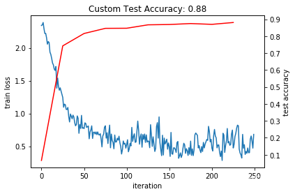
_, ax1 = subplots()
ax2 = ax1.twinx()
ax1.plot(arange(niter), train_loss)
ax2.plot(test_interval*arange(len(test_acc)), test_acc, 'r')
ax1.set_xlabel('iteration')
ax1.set_ylabel('train loss')
ax2.set_ylabel('test accuracy')
ax2.set_title('Custom Test Accuracy: {:.2f}'.format(test_acc[-1]))    

Text(0.5, 1.0, 'Custom Test Accuracy: 0.88')

理解总结部分

1. 通常情况下，caffe在训练和测试网络时，需要借助对应的prototxt文件，一个是定义网络结构和输入数据的net prototxt文件，net prototxt文件又分为train prototxt和test prototxt。还有一个solver prototxt，用来定义一些超参数，例如Learning rate， weights decay， momentum，还有lr_policy等

2. test_iter和test_interval的区别

test_iter是指测试需要迭代的次数，如果有10000张测试图片，batch_size=100的情况下，test_iter=100能覆盖满整个数据集
test_interval是指进行玩对应次数训练后，进行一次测试，假如test_interval = 500，表示进行500次训练后进行一次测试

3. solver.step(1)

进行一次（minibatch）SGD的操作

4.snapshot 用来保存中间结果

5.lr_policy有哪些？

// The learning rate decay policy. The currently implemented learning rate
  // policies are as follows:
  //    - fixed: always return base_lr.
  //    - step: return base_lr * gamma ^ (floor(iter / step))
  //    - exp: return base_lr * gamma ^ iter
  //    - inv: return base_lr * (1 + gamma * iter) ^ (- power)
  //    - multistep: similar to step but it allows non uniform steps defined by
  //      stepvalue
  //    - poly: the effective learning rate follows a polynomial decay, to be
  //      zero by the max_iter. return base_lr (1 - iter/max_iter) ^ (power)
  //    - sigmoid: the effective learning rate follows a sigmod decay
  //      return base_lr ( 1/(1 + exp(-gamma * (iter - stepsize))))
  //
  // where base_lr, max_iter, gamma, step, stepvalue and power are defined
  // in the solver parameter protocol buffer, and iter is the current iteration.
  optional string lr_policy = 8;
  optional float gamma = 9; // The parameter to compute the learning rate.
  optional float power = 10; // The parameter to compute the learning rate.
  optional float momentum = 11; // The momentum value.
  optional float weight_decay = 12; // The weight decay.

6. 有哪些优化方式？

// type of the solver
  optional string type = 40 [default = "SGD"];

  // numerical stability for RMSProp, AdaGrad and AdaDelta and Adam
  optional float delta = 31 [default = 1e-8];
  // parameters for the Adam solver
  optional float momentum2 = 39 [default = 0.999];

  // RMSProp decay value
  // MeanSquare(t) = rms_decay*MeanSquare(t-1) + (1-rms_decay)*SquareGradient(t)
  optional float rms_decay = 38 [default = 0.99];

  // If true, print information about the state of the net that may help with
  // debugging learning problems.
  optional bool debug_info = 23 [default = false];

  // If false, don't save a snapshot after training finishes.
  optional bool snapshot_after_train = 28 [default = true];

  // DEPRECATED: old solver enum types, use string instead
  enum SolverType {
    SGD = 0;
    NESTEROV = 1;
    ADAGRAD = 2;
    RMSPROP = 3;
    ADADELTA = 4;
    ADAM = 5;
  }
  // DEPRECATED: use type instead of solver_type
  optional SolverType solver_type = 30 [default = SGD];

参考地址：
https://nbviewer.jupyter.org/github/BVLC/caffe/blob/master/examples/01-learning-lenet.ipynb