霍夫变换
opencv 霍夫直线变换
OpenCV中用cv.HoughLines()在二值图上实现霍夫变换,函数返回的是一组直线的(r,θ)数据:
函数中:
参数1:要检测的二值图(一般是阈值分割或边缘检测后的图)
参数2:距离r的精度,值越大,考虑越多的线
参数3:角度θ的精度,值越小,考虑越多的线
参数4:累加数阈值,值越小,考虑越多的线
实验:检测图像中的直线
import cv2 as cv
import numpy as np

# 1. 霍夫直线变换
img = cv.imread('shapes.jpg')
drawing = np.zeros(img.shape[:], dtype=np.uint8)  # 创建画板
gray = cv.cvtColor(img, cv.COLOR_BGR2GRAY)
edges = cv.Canny(gray, 50, 150)

# 霍夫直线变换
lines = cv.HoughLines(edges, 0.8, np.pi / 180, 90)

# 将检测的线画出来(注意是极坐标噢)
for line in lines:
    rho, theta = line[0]
    a = np.cos(theta)
    b = np.sin(theta)
    x0 = a * rho
    y0 = b * rho
    x1 = int(x0 + 1000 * (-b))
    y1 = int(y0 + 1000 * (a))
    x2 = int(x0 - 1000 * (-b))
    y2 = int(y0 - 1000 * (a))

    cv.line(drawing, (x1, y1), (x2, y2), (0, 0, 255))

cv.imshow('hough lines', np.hstack((img, drawing)))
cv.waitKey(0)
实验结果
统计概率霍夫直线变换
前面的方法又称为标准霍夫变换,它会计算图像中的每一个点,计算量比较大,另外它得到的是整一条线(r和θ),并不知道原图中直线的端点。所以提出了统计概率霍夫直线变换(Probabilistic Hough Transform),是一种改进的霍夫变换:
drawing = np.zeros(img.shape[:], dtype=np.uint8)
# 统计概率霍夫线变换
lines = cv.HoughLinesP(edges, 0.8, np.pi / 180, 90,
                        minLineLength=50,   maxLineGap=10)
前面几个参数跟之前的一样,有两个可选参数:
minLineLength:最短长度阈值,比这个长度短的线会被排除
maxLineGap:同一直线两点之间的最大距离
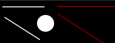
实验:统计概率霍夫直线变换检测图像中的直线
import cv2 as cv
import numpy as np

# 1. 霍夫直线变换
img = cv.imread('shapes.jpg')
drawing = np.zeros(img.shape[:], dtype=np.uint8)  # 创建画板
gray = cv.cvtColor(img, cv.COLOR_BGR2GRAY)
edges = cv.Canny(gray, 50, 150)

# 霍夫直线变换
lines = cv.HoughLinesP(edges, 0.8, np.pi / 180, 90, minLineLength=50, maxLineGap=10)

# 将检测的线画出来
for line in lines:
	x1, y1, x2, y2 = line[0]
	cv.line(drawing, (x1, y1), (x2, y2), (255, 0, 0), 1, lineType=cv.LINE_AA)

cv.imshow('probabilistic hough lines', np.hstack((img, drawing)))
cv.waitKey(0)
实验结果

霍夫圆变换
霍夫圆变换跟直线变换类似,只不过线是用(r,θ)表示,圆是用(x_center,y_center,r)来表示,从二维变成了三维,数据量变大了很多;所以一般使用霍夫梯度法减少计算量。
drawing = np.zeros(img.shape[:], dtype=np.uint8)
# 霍夫圆变换
circles = cv.HoughCircles(edges, cv.HOUGH_GRADIENT, 1, 20, param2=30)
circles = np.int0(np.around(circles))
参数2:变换方法,一般使用霍夫梯度法,详情:HoughModes
参数3:dp=1:表示霍夫梯度法中累加器图像的分辨率与原图一致
参数4:两个不同圆圆心的最短距离
参数5:param2跟霍夫直线变换中的累加数阈值一样
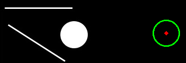
实验:霍夫圆变换检测图像中的圆
import cv2 as cv
import numpy as np

img = cv.imread('shapes.jpg')
drawing = np.zeros(img.shape[:], dtype=np.uint8)  # 创建画板
gray = cv.cvtColor(img, cv.COLOR_BGR2GRAY)
edges = cv.Canny(gray, 50, 150)

# 霍夫圆变换
circles = cv.HoughCircles(edges, cv.HOUGH_GRADIENT, 1, 20, param2=30)
circles = np.int0(np.around(circles))

# 将检测的圆画出来
for i in circles[0, :]:
    cv.circle(drawing, (i[0], i[1]), i[2], (0, 255, 0), 2)  # 画出外圆
    cv.circle(drawing, (i[0], i[1]), 2, (0, 0, 255), 3)  # 画出圆心

cv.imshow('circles', np.hstack((img, drawing)))
cv.waitKey(0)
实验结果