1 原理
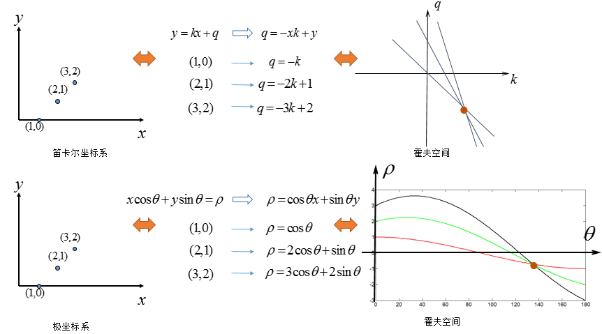
1.众所周知, 一条直线在图像二维空间可由两个变量表示. 例如:
在 笛卡尔坐标系: 可由参数:
斜率和截距表示.
在 极坐标系: 可由参数:
极径和极角表示
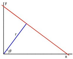
对于霍夫变换, 我们将用 极坐标系 来表示直线. 因此, 直线的表达式可为:
化简得:
2.一般来说对于点 , 我们可以将通过这个点的一族直线统一定义为:
这就意味着每一对 代表一条通过点 的直线.
3.如果对于一个给定点 我们在极坐标对极径极角平面绘出所有通过它的直线, 将得到一条正弦曲线. 例如, 对于给定点 和 我们可以绘出下图 (在平面 ):
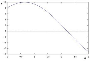
只绘出满足下列条件的点
.
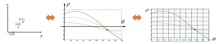
4.我们可以对图像中所有的点进行上述操作. 如果两个不同点进行上述操作后得到的曲线在平面
相交, 这就意味着它们通过同一条直线. 例如, 接上面的例子我们继续对点:
和点
绘图, 得到下图:
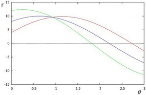
这三条曲线在
平面相交于点
, 坐标表示的是参数对
或者是说点
, 点
和点
组成的平面内的的直线.
5.那么以上的材料要说明什么呢? 这意味着一般来说, 一条直线能够通过在平面 寻找交于一点的曲线数量来 检测. 越多曲线交于一点也就意味着这个交点表示的直线由更多的点组成. 一般来说我们可以通过设置直线上点的 阈值 来定义多少条曲线交于一点我们才认为 检测 到了一条直线.
6.这就是霍夫线变换要做的. 它追踪图像中每个点对应曲线间的交点. 如果交于一点的曲线的数量超过了 阈值, 那么可以认为这个交点所代表的参数对 在原图像中为一条直线.
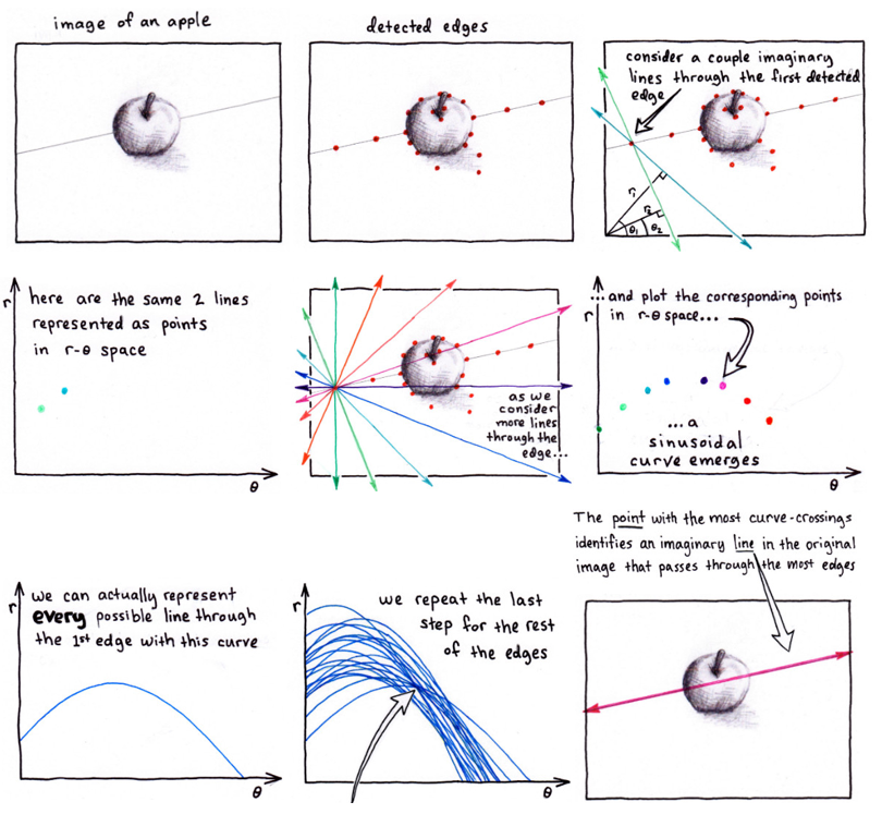
另一种解释:
首先,介绍笛卡尔空间,就是我们常见的那个几何空间啦,通过 ,可以表示直线。
然后,想一下,如果把上面方程变形一下, ,(k和b作为变量,xy作为常量),那么是不是又是一条另外的直线呢?对了,这就是霍夫空间了。
然后,你一不小心,发现两个规律:
①霍夫空间,笛卡尔空间中的直线,对应到霍夫空间中是一个点;
②笛卡尔空间中共线的点,在霍夫空间中对应的直线相交。(这个很重要,因为在笛卡尔空间中,我要做直线检测,岂不就是要找到最多的点所在的那条线嘛,我把所有的点都映射到霍夫空间中,找到最多的线公共交点就可以了。)
再然后,你会发现一个问题,如果是一条垂直于x轴的直线,那么k岂不是正无穷,怎么办?
没关系,引进极坐标表示直线: ( 为原点到直线的距离),如图所示:
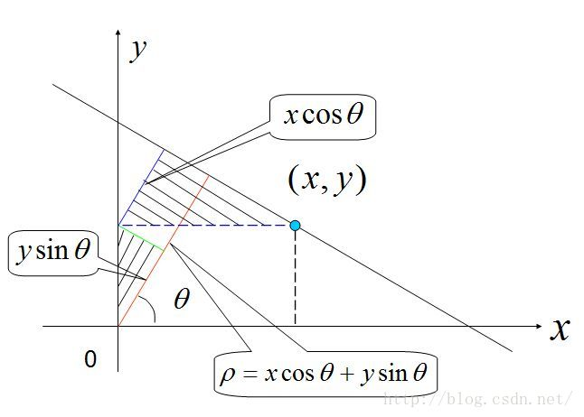
再然后,就可以将笛卡尔空间和霍夫空间做映射了。
总结下上面的过程,如下图:
继续然后,上面红色字体:找到最多的线公共交点就可以了,怎么找?
哈哈,直接小白方式寻找,把霍夫空间网格化(就是一个很大的矩阵,初始值全是0),直线经过的地方标注1,没经过的地方还是0。再找出值最大的一些点就可以了。
①对其进行边缘检测
②边缘检测后并二值化,就可以通过找非零点的坐标确定数据点
③对数据点进行霍夫变换,就形成了下面那个第三个图,好像一个水管,其实是很多很多曲线组成
④找出其中数值较大的一些点,通常可以给定一个阈值,Threshold一下,上面不是说了嘛,数值较大的点(我用红框框出来了)说明对应笛卡尔空间共线。
⑤最后得到那个有彩色直线的图,完成了直线检测。
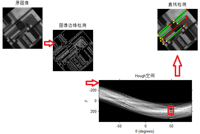
上面的过程讲述原理,到此结束,算了,再举个栗子吧:
2 检测直线
其中基本的版本是cv2.HoughLines。其输入一幅含有点集的二值图(由非0像素表示),其中一些点互相联系组成直线。通常这是通过如Canny算子获得的一幅边缘图像。cv2.HoughLines函数输出的是[float, float]形式的ndarray,其中每个值表示检测到的线(ρ , θ)中浮点点值的参数。下面的例子首先使用Canny算子获得图像边缘,然后使用Hough变换检测直线。其中HoughLines函数的参数3和4对应直线搜索的步长。在本例中,函数将通过步长为1的半径和步长为π/180的角来搜索所有可能的直线。最后一个参数是经过某一点曲线的数量的阈值,超过这个阈值,就表示这个交点所代表的参数对(rho, theta)在原图像中为一条直线。
通过HoughLines()和HoughLinesP()函数来完成。两者主要区别:前者使用标准的Hough变换,后者使用概率Hough变换(因此名称里有一个字母’P’)
HoughLinesP()函数之所以称为概率版本的Hough变换是因为它只通过分析点的子集并估计这些点都属于一条直线的概率,这就是标准Hough变换的优化版本。
使用HoughLines()检测直线
cv2.HoughLines(image, rho, theta, threshold[, lines[, srn[, stn[, min_theta[, max_theta]]]]]) → lines
-
image – 8-bit, single-channel binary source image. The image may be modified by the function.
-
rho – Distance resolution of the accumulator in pixels.
-
theta – Angle resolution of the accumulator in radians( 弧度角).
-
threshold – Accumulator threshold parameter. Only those lines are returned that get enough votes ( >threshold).
-
lines – Output vector of lines. Each line is represented by a 2 or 3 element vector or . is the distance from the coordinate origin (top-left corner of the image). is the line rotation angle in radians. is the value of accumulator.
import cv2
import numpy as np

img = cv2.imread('lines.png')
h, w = img.shape
gray = cv2.cvtColor(img,cv2.COLOR_BGR2GRAY)
edges = cv2.Canny(gray,50,150)

#200 代表应该检测到的行的最小长度
lines = cv2.HoughLines(edges, 1, np.pi/180, 200)

for i in range(len(lines)):
    for rho,theta in lines[i]:
        a = np.cos(theta)
        b = np.sin(theta)
        x0 = a*rho
        y0 = b*rho
        x1 = int(x0 + w*(-b))
        y1 = int(y0 + w*(a))
        x2 = int(x0 - w*(-b))
        y2 = int(y0 - w*(a))

        cv2.line(img,(x1,y1),(x2,y2),(0,0,255),2)
cv2.imshow("edges",edges)
cv2.imshow("lines", img)
cv2.waitKey()
cv2.destroyAllWindows()
#lines本身
(1, 5, 2) #lines.shape属性
[[[ 4.20000000e+01 2.14675498e+00]
[ 4.50000000e+01 2.14675498e+00]
[ 3.50000000e+01 2.16420817e+00]
[ 1.49000000e+02 1.60570288e+00]
[ 2.24000000e+02 1.74532920e-01]]]
使用HoughLinesP()检测直线
cv2.HoughLinesP(image, rho, theta, threshold[, lines[, minLineLength[, maxLineGap]]]) → lines
- image – 8-bit, single-channel binary source image. The image may be modified by the function.
- rho – Distance resolution of the accumulator in pixels.
- theta – Angle resolution of the accumulator in radians.
- threshold – Accumulator threshold parameter. Only those lines are returned that get enough votes ( >threshold ).
- minLineLength – Minimum line length. Line segments shorter than that are rejected.
- maxLineGap – Maximum allowed gap between points on the same line to link them.
import cv2
import numpy as np

img = cv2.imread('lines.png')

gray = cv2.cvtColor(img,cv2.COLOR_BGR2GRAY)
edges = cv2.Canny(gray,50,150)


#最低线段的长度,小于这个值的线段被抛弃
minLineLength = 100

#线段中点与点之间连接起来的最大距离,在此范围内才被认为是单行
maxLineGap =10

#100阈值,累加平面的阈值参数,即:识别某部分为图中的一条直线时它在累加平面必须达到的值,低于此值的直线将被忽略。
lines = cv2.HoughLinesP(edges, 1, np.pi/180, 100, minLineLength, maxLineGap)

for i in range(len(lines)):
    for x1,y1,x2,y2 in lines[i]:
        cv2.line(img, (x1,y1), (x2,y2), (0,255,0), 2)

cv2.imshow("edges",edges)
cv2.imshow("lines", img)
cv2.waitKey()
cv2.destroyAllWindows()
reference:
https://www.cnblogs.com/dyllove98/archive/2013/07/12/3186872.html
http://www.opencv.org.cn/opencvdoc/2.3.2/html/doc/tutorials/imgproc/imgtrans/hough_lines/hough_lines.html
https://blog.csdn.net/cc1949/article/details/79747205
https://blog.csdn.net/cc1949/article/details/79747205
