python-opencv 图像处理基础 （九）图像梯度+边缘检测+直线检测+圆检测+轮廓检测+对象测量

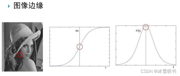
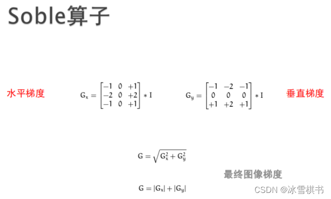
一阶导数与sobel算子
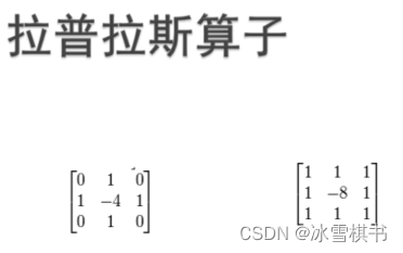
二阶导数与拉普拉斯算子
其它边缘算子—边缘检测、直线检测

一阶导数与sobel算子

二阶导数和拉普拉斯算子

在二阶导数的时候，最大变化处的值为0即边缘是零值。通过二阶导数计算，依据此理论可以计算图像二阶导数，提取边缘。

import cv2 as cv
import numpy as np


def lapalian_demo(image):
    #第一种方法调用算子
    #dst = cv.Laplacian(image, cv.CV_32F)
    #lpls = cv.convertScaleAbs(dst)

    #第二种方法手动实现
    kernel = np.array([[1, 1, 1], [1, -8, 1], [1, 1, 1]])#定义卷积核 8邻域 还可以4邻域
    dst = cv.filter2D(image, cv.CV_32F, kernel=kernel)
    lpls = cv.convertScaleAbs(dst)
    cv.imshow("lapalian_demo", lpls)


def sobel_demo(image):
    # grad_x = cv.Sobel(image, cv.CV_32F, 1, 0)#32位float浮点数 不能使用8u 加加减减超256了。
    # grad_y = cv.Sobel(image, cv.CV_32F, 0, 1)
    grad_x = cv.Scharr(image, cv.CV_32F, 1, 0)  #Scharr边缘增强，对弱边缘梯度提取效果好
    grad_y = cv.Scharr(image, cv.CV_32F, 0, 1)
    gradx = cv.convertScaleAbs(grad_x)
    grady = cv.convertScaleAbs(grad_y)
    cv.imshow("gradient-x", gradx)
    cv.imshow("gradient-y", grady)

    gradxy = cv.addWeighted(gradx, 0.5, grady, 0.5, 0)
    cv.imshow("gradient", gradxy)


if __name__=='__main__':
    print("--------- Python OpenCV Tutorial ---------")
    src = cv.imread("../opencv-python-img/lena.png")
    cv.namedWindow("input image", cv.WINDOW_AUTOSIZE)
    cv.imshow("input image", src)
    #sobel_demo(src)
    lapalian_demo(src)
    cv.waitKey(0)

cv.destroyAllWindows()

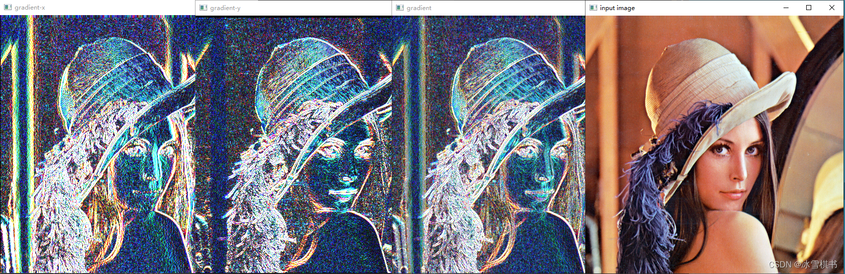
sobel_demo的result显示：
上下和左右的差异
x和y方向最终结果很好的反应了像素梯度变化差异

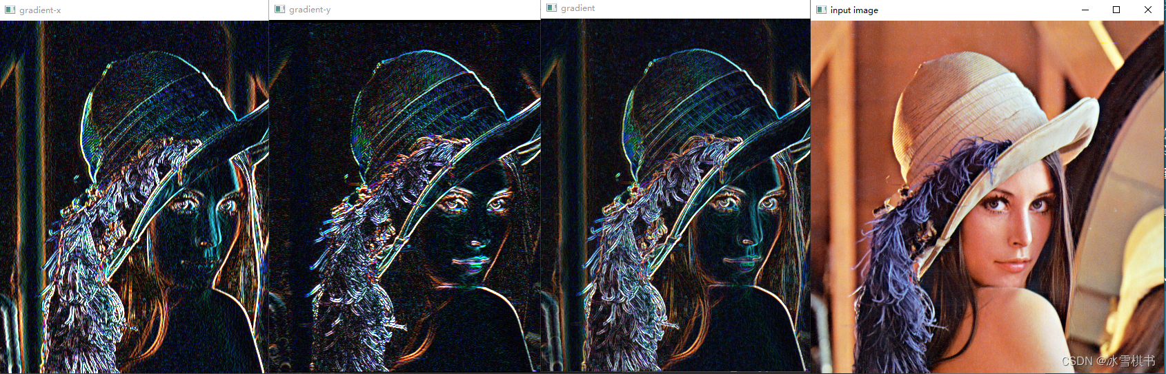scharr 进行边缘增强后的梯度提取，提取弱边缘 ，噪声敏感，需要降噪
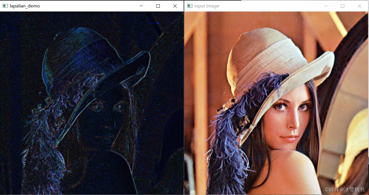
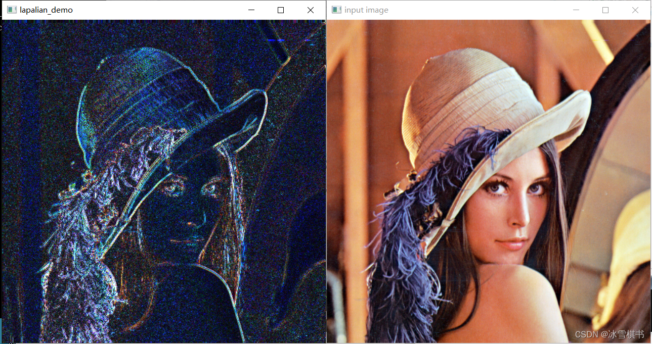
拉普拉斯的结果输出：
直接调用算子的结果：

手动卷积实现的结果

其它边缘提取算子

canny边缘提取

canny：边缘检测算法，1986年提出的。
是一个很好的边缘检测器
很常用也很实用的图像处理方法

步骤：

	高斯模糊--GaussianBlur   为什么：因为canny对边缘噪声敏感
	灰度转换--CVTColor
	计算梯度--sobel/scharr
	非最大信号抑制
	高低阈值输出二值图像

import cv2 as cv
import numpy as np


def edge_demo(image):
    blurred = cv.GaussianBlur(image, (3, 3), 0)
    gray = cv.cvtColor(blurred, cv.COLOR_BGR2GRAY)
    # X Gradient
    xgrad = cv.Sobel(gray, cv.CV_16SC1, 1, 0)
    # Y Gradient
    ygrad = cv.Sobel(gray, cv.CV_16SC1, 0, 1)
    #edge
    #edge_output = cv.Canny(xgrad, ygrad, 50, 150)
    edge_output = cv.Canny(gray, 50, 150)
    cv.imshow("Canny Edge", edge_output)

    dst = cv.bitwise_and(image, image, mask=edge_output)
    cv.imshow("Color Edge", dst)

if __name__=='__main__':
    print("--------- Python OpenCV Tutorial ---------")
    src = cv.imread("../opencv-python-img/lena.png")
    cv.namedWindow("input image", cv.WINDOW_AUTOSIZE)
    cv.imshow("input image", src)
    edge_demo(src)
    cv.waitKey(0)

    cv.destroyAllWindows()

使用sobel的x和y梯度提取边缘

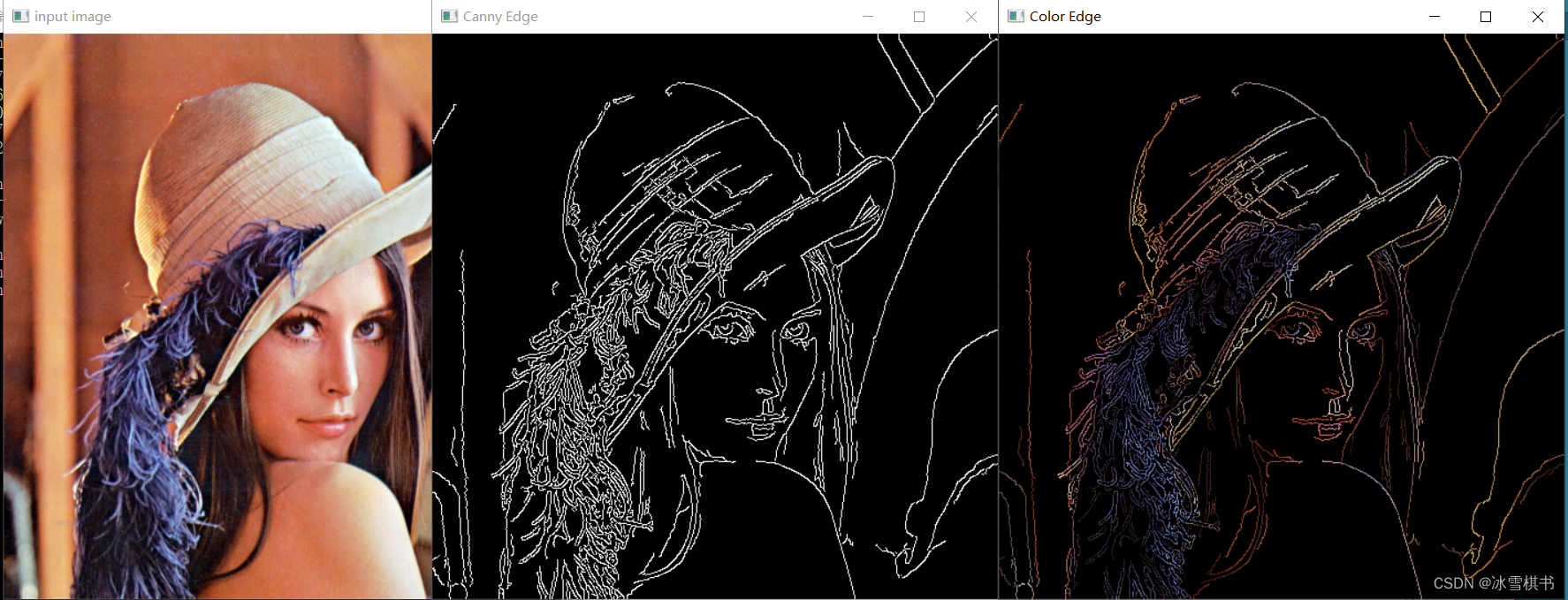
使用灰度图提取canny边缘：

霍夫直线检测

Hough Line Transform 用来做直线检测
前提条件：边缘检测已经完成
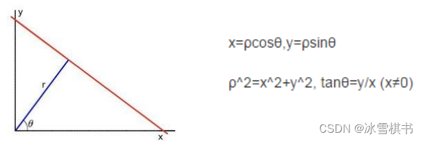
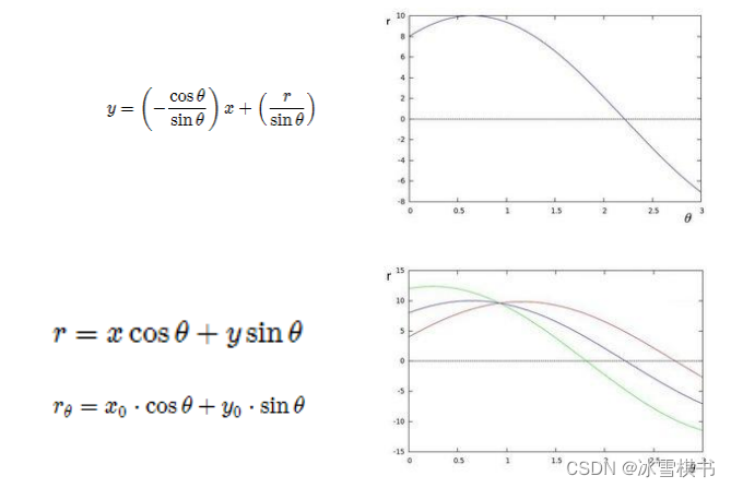
平面空间到极坐标空间转换

import cv2 as cv
import numpy as np


def line_detection(image):
    gray = cv.cvtColor(image, cv.COLOR_BGR2GRAY)
    edges = cv.Canny(gray, 50, 150, apertureSize=3)#做梯度窗口的大小是3.
    lines = cv.HoughLines(edges, 1, np.pi/180, 200) #1是半径步长，np.pi/180每次偏转1度，
    for line in lines:
        print(type(lines))
        rho, theta = line[0]
        a = np.cos(theta)
        b = np.sin(theta)
        x0 = a * rho
        y0 = b * rho
        x1 = int(x0+1000*(-b))
        y1 = int(y0+1000*(a))
        x2 = int(x0-1000*(-b))
        y2 = int(y0-1000*(a))
        cv.line(image, (x1, y1), (x2, y2), (0, 0, 255), 2)
    cv.imshow("image-lines", image)


def line_detect_possible_demo(image):
    gray = cv.cvtColor(image, cv.COLOR_BGR2GRAY)
    edges = cv.Canny(gray, 50, 150, apertureSize=3)
    lines = cv.HoughLinesP(edges, 1, np.pi/180, 100, minLineLength=50, maxLineGap=10)#常用这个API，会告诉我们线段的开始点和终止点
    for line in lines:
        print(type(line))
        x1, y1, x2, y2 = line[0]
        cv.line(image, (x1, y1), (x2, y2), (0, 0, 255), 2)
    cv.imshow("line_detect_possible_demo", image)


if __name__=='__main__':
    print("--------- Python OpenCV Tutorial ---------")
    src = cv.imread("../opencv-python-img/test.png")
    cv.namedWindow("input image", cv.WINDOW_AUTOSIZE)
    cv.imshow("input image", src)
    line_detect_possible_demo(src)
    cv.waitKey(0)

    cv.destroyAllWindows()

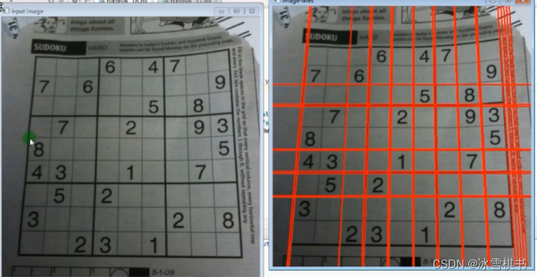
使用HoughLines函数的结果显示：

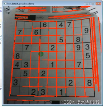
使用HoughLinesP 函数的结果显示：这个API常用。

霍夫圆检测

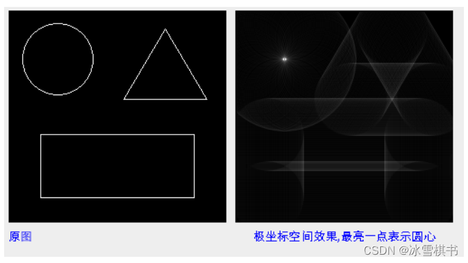
因为霍夫圆检测对噪声比较敏感，所以首先要对图像做中值滤波。
基于效率考虑，Opencv中实现的霍夫变换圆检测是基于图像梯度的实现，分为两步：

1. 检测边缘，发现可能的圆心
2. 基于第一步的基础上从候选圆心开始计算最佳半径大小

import cv2 as cv
import numpy as np


def detect_circles_demo(image):
    dst = cv.pyrMeanShiftFiltering(image, 10, 100)#基于边缘保留的滤波
    cimage = cv.cvtColor(dst, cv.COLOR_BGR2GRAY)
    circles = cv.HoughCircles(cimage, cv.HOUGH_GRADIENT, 1, 20, param1=50, param2=30, minRadius=0, maxRadius=0)
    circles = np.uint16(np.around(circles))#整数
    for i in circles[0, :]:
        cv.circle(image, (i[0], i[1]), i[2], (0, 0, 255), 2)#图像，中心点位置，半径，颜色，线宽
        cv.circle(image, (i[0], i[1]), 2, (255, 0, 0), 2)#圆心
    cv.imshow("circles", image)


if __name__=='__main__':
    print("--------- Python OpenCV Tutorial ---------")
    src = cv.imread("../opencv-python-img/coins.jpg")
    cv.namedWindow("input image", cv.WINDOW_AUTOSIZE)
    cv.imshow("input image", src)
    detect_circles_demo(src)
    cv.waitKey(0)

    cv.destroyAllWindows()

代码结果显示：

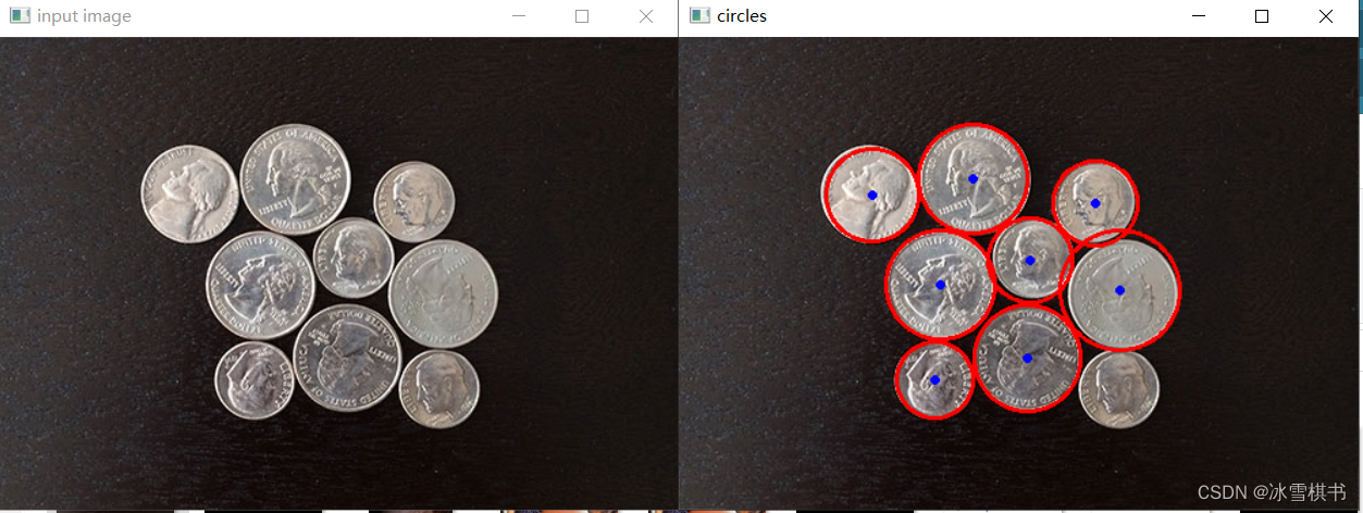
霍夫圆检测的实例

钢管检测：个人总结

轮廓检测

轮廓发现

是基于图像边缘提取的基础寻找对象轮廓的方法。
所以边缘提取的阈值选定会影响最终轮廓发现结果

API介绍

-findContours发现轮廓
-drawContours绘制轮廓

API利用梯度来避免阈值烦恼

原图直接找轮廓有噪点：

高斯模糊去噪点dst = cv.GaussianBlur(image, (3, 3), 0)：

cv.RETR_TREE 内外轮廓都找（cv2.findContours(binary, cv.RETR_TREE, cv.CHAIN_APPROX_SIMPLE)）
cv.RETR_EXTERNAL找外轮廓cv2.findContours(binary, cv.RETR_EXTERNAL, cv.CHAIN_APPROX_SIMPLE)

填充轮廓cv.drawContours(image, contours, i, (0, 0, 255), -1)
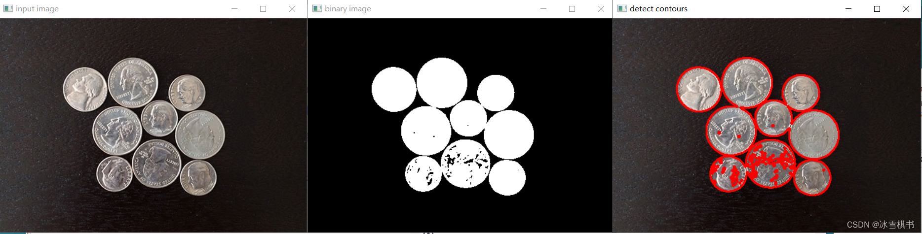
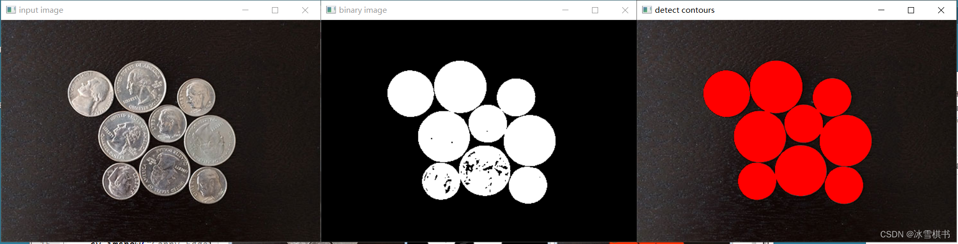通过canny 获取轮廓：不是想要的结果，根据情况选择，这种硬币的轮廓提取使用二值化提取。

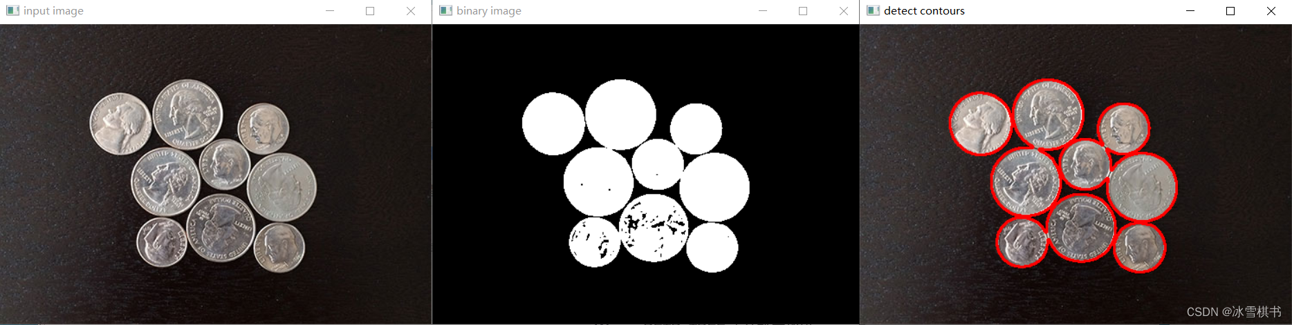
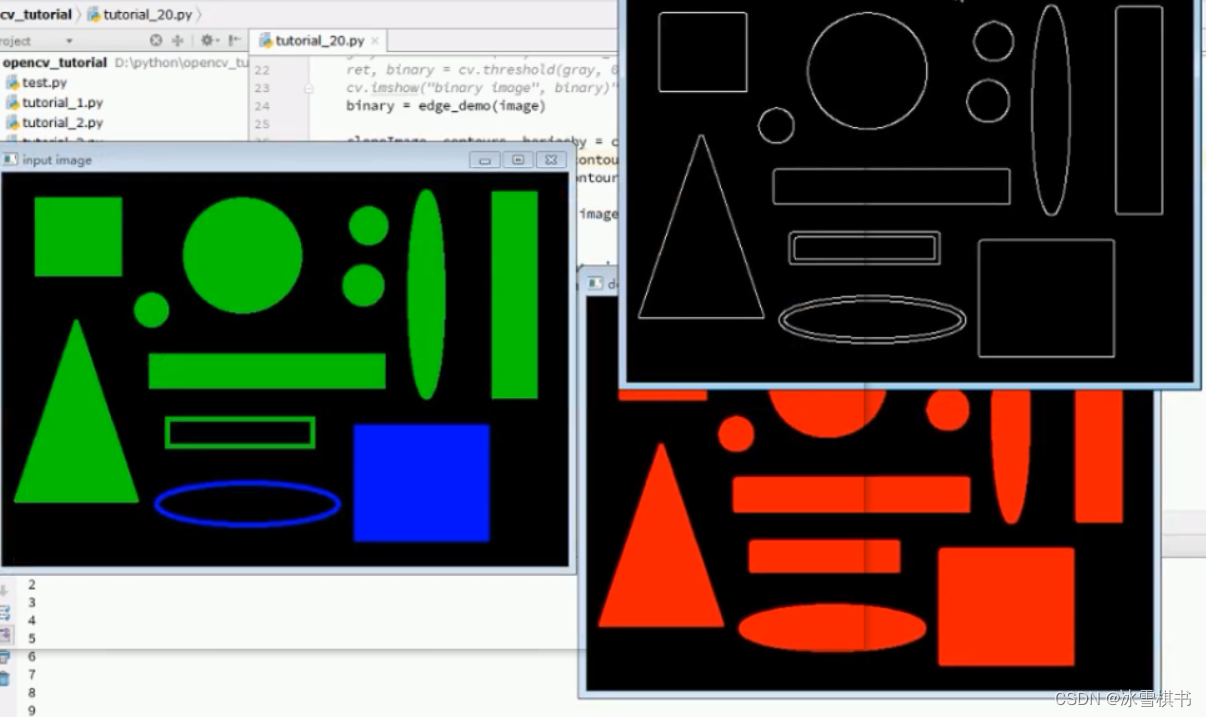
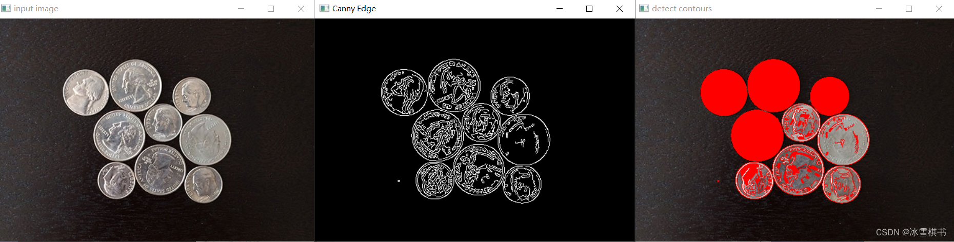以下示例使用canny获取轮廓效果好：适当调整canny的参数

import cv2 as cv
import numpy as np


def edge_demo(image):
    blurred = cv.GaussianBlur(image, (3, 3), 0)
    gray = cv.cvtColor(blurred, cv.COLOR_BGR2GRAY)
    # X Gradient
    xgrad = cv.Sobel(gray, cv.CV_16SC1, 1, 0)
    # Y Gradient
    ygrad = cv.Sobel(gray, cv.CV_16SC1, 0, 1)
    #edge
    #edge_output = cv.Canny(xgrad, ygrad, 50, 150)
    edge_output = cv.Canny(gray, 50, 150)
    cv.imshow("Canny Edge", edge_output)
    return edge_output


def contours_demo(image):
    #第一种方法获取二值图像
    #dst = cv.GaussianBlur(image, (3, 3), 0)#去除噪点
    #gray = cv.cvtColor(dst, cv.COLOR_BGR2GRAY)
    #ret, binary = cv.threshold(gray, 0, 255, cv.THRESH_BINARY | cv.THRESH_OTSU)
    #cv.imshow("binary image", binary)
    #第二种方法通过canny 获取二值图像
    binary = edge_demo(image)

    #cloneImage, contours, heriachy = cv.findContours(binary, cv.RETR_EXTERNAL, cv.CHAIN_APPROX_SIMPLE)
    #contours, heriachy = cv.findContours(binary, cv.RETR_TREE, cv.CHAIN_APPROX_SIMPLE)#内外的轮廓都找
    contours, heriachy = cv.findContours(binary, cv.RETR_EXTERNAL, cv.CHAIN_APPROX_SIMPLE)#找外面的轮廓

    for i, contour in enumerate(contours):
        #cv.drawContours(image, contours, i, (0, 0, 255), 2)#
        cv.drawContours(image, contours, i, (0, 0, 255), -1)#轮廓填充

        print(i)
    cv.imshow("detect contours", image)


if __name__=='__main__':
    print("--------- Python OpenCV Tutorial ---------")
    src = cv.imread("../opencv-python-img/coins.jpg")
    cv.namedWindow("input image", cv.WINDOW_AUTOSIZE)
    cv.imshow("input image", src)
    contours_demo(src)
    cv.waitKey(0)

    cv.destroyAllWindows()

对象测量

• 弧长与面积
  轮廓发现
  计算每个轮廓的弧长和面积，像素单位
• 多边形拟合
• 几何矩计算

import cv2 as cv
import numpy as np
#轮廓分析 计算轮廓面积和轮廓几何
#区分不同的几何形状，圆形 四边形等
def measure_object(image):
    image = cv.GaussianBlur(image, (3, 3), 0)
    gray = cv.cvtColor(image, cv.COLOR_BGR2GRAY)
    #ret, binary = cv.threshold(gray, 0, 255, cv.THRESH_BINARY | cv.THRESH_OTSU)#
    ret, binary = cv.threshold(gray, 0, 255, cv.THRESH_BINARY_INV | cv.THRESH_OTSU)#取反

    print("threshold value : %s"%ret)
    cv.imshow("binary image", binary)
    dst = cv.cvtColor(binary, cv.COLOR_GRAY2BGR)
    contours, hireachy = cv.findContours(binary, cv.RETR_EXTERNAL, cv.CHAIN_APPROX_SIMPLE)
    for i, contour in enumerate(contours):
        area = cv.contourArea(contour)#求轮廓的面积，得到第几个轮廓的面积
        x, y, w, h = cv.boundingRect(contour)#轮廓的外接矩形的大小，
        rate = min(w, h)/max(w, h)
        print("rectangle rate : %s"%rate)
        mm = cv.moments(contour)#得到contour的几何矩
        print(type(mm))#dict字典类型
        cx = mm['m10']/mm['m00']
        cy = mm['m01']/mm['m00']
        cv.circle(dst, (np.int(cx), np.int(cy)), 3, (0, 255, 255), -1)
        cv.rectangle(dst, (x, y), (x+w, y+h), (0, 0, 255), 2)#每个轮廓绘制外接矩形
        print("contour area %s"%area)
        approxCurve = cv.approxPolyDP(contour,4, True)#对指定的点集进行逼近 找出轮廓的多边形拟合曲线
        print(approxCurve.shape)
        if approxCurve.shape[0] > 6:
            cv.drawContours(dst, contours, i, (0, 255, 0), 2)
        if approxCurve.shape[0] == 4:
            cv.drawContours(dst, contours, i, (0, 0, 255), 2)
        if approxCurve.shape[0] == 3:
            cv.drawContours(dst, contours, i, (255, 0, 0), 2)
    cv.imshow("measure-contours", dst)


print("--------- Python OpenCV Tutorial ---------")
src = cv.imread("../opencv-python-img/coins.jpg")
cv.namedWindow("input image", cv.WINDOW_AUTOSIZE)
cv.imshow("input image", src)
measure_object(src)
cv.waitKey(0)

cv.destroyAllWindows()