一:更改色彩空间(一共150多种)
对于颜色转换,我们使用函数cv2.cvtColor(input_image,flag),其中flag确定转换类型。
对于BGR Gray转换,我们使用标志cv2.COLOR_BGR2GRAY。类似地,对于BGR HSV,我们使用标志cv2.COLOR_BGR2HSV。要获取其他标志,只需在Python终端中运行以下命令:→→
 import cv2
flags = [c for c in dir(cv2) if c.startswith('COLOR_')]
print (flags)

二:对象追踪
• 拍摄视频的每一帧
• 从BGR转换为HSV色彩空间
• 我们将HSV图像阈值为一系列蓝色
• 现在单独提取蓝色对象,我们可以对我们想要的图像做任何事情。
import cv2
#flags = [i for i in dir(cv2) if i.startswith('COLOR_')]
#print (flags)
import numpy as np
cap = cv2.VideoCapture(0)
while(1):
#拍摄每一帧
    _,frame = cap.read()
#将BGR转换为HSV
    hsv = cv2.cvtColor (frame,cv2.COLOR_BGR2HSV)
#defn定义HSV中的蓝色范围
    lower_blue = np.array ([110,50,50])
    upper_blue = np.array ([120,255,255])
#阈值HSV图像仅获得蓝色
    mask = cv2.inRange (hsv, lower_blue, upper_blue)
#Bitwise-AND掩码和原始图像
    res = cv2.bitwise_and (frame, frame, mask = mask)
    cv2.imshow ('frame',frame)
    cv2.imshow('mask',mask)
    cv2.imshow('res',res)
    k = cv2.waitKey (5) & 0xFF
    if k ==27:
        break
cv2.destroyAllWindows()

三:图像的几何变换
转换提供了两个转换函数cv2.warpAffine和cv2.warpPerspective,其中cv2.warpAffine采用2x3变换矩阵,而cv2.warpPerspective采用3x3变换矩阵作为输入。
缩放 调整图像大小,cv2.resize(), 优选的内插方法是cv2.INTER_AREA用于收缩和cv2.INTER_CUBIC(慢)cv2.INTER_LINEAR用于变焦。默认情况下,使用的插值方法是cv2.INTER_LINEAR,用于所有调整大小的目的
旋转
import numpy as np
import cv2
def main():
    img = cv2.imread('.\\imgs\\img10.jpg')
    height, width = img.shape[:2]

    matRotate = cv2.getRotationMatrix2D((height * 0.5, width * 0.5), -90, 1)
    dst = cv2.warpAffine(img, matRotate, (width, height*2))
    rows, cols = dst.shape[:2]

    for col in range(0, cols):
        if dst[:, col].any():
            left = col
            break

    for col in range(cols-1, 0, -1):
        if dst[:, col].any():
            right = col
            break

    for row in range(0, rows):
        if dst[row,:].any():
            up = row
            break

    for row in range(rows-1,0,-1):
        if dst[row,:].any():
            down = row
            break

    res_widths = abs(right - left)
    res_heights = abs(down - up)
    res = np.zeros([res_heights ,res_widths, 3], np.uint8)

    for res_width in range(res_widths):
        for res_height in range(res_heights):
            res[res_height, res_width] = dst[up+res_height, left+res_width]

    cv2.imshow('res',res)

    cv2.imshow('img',img)
    cv2.imshow('dst', dst)
    cv2.waitKey(0)

if __name__ =='__main__':
    main()

四。图像的阈值
阈值就是最简单的图像的分割法
1.简单的阈值(如果像素值大于阈值,则为其分配一个值(可以是白色),否则为其分配另一个值(可以是黑色)
cv2.threshold(源图像也就是灰度图像,对像素值进行分类的阈值,maxVal表示如果像素值大于(有时小于)阈值则要给出的值)
ret, dst = threshold(src, thresh, maxval, type)
ret: retVal(返回值),在Otsu‘s中会用到
dst: 目标图像
src: 原图像,只能输入单通道图像,通常来说为灰度图
thresh: 阈值
maxval: 当像素值超过了阈值(或者小于阈值,根据type来决定),所赋予的值
type:阈值类型,包含以下5种类型:1.二进制阈值化:cv2.THRESH_BINARY ,大于阈值取maxval,小于取0
2.反二进制阈值化:cv2.THRESH_BINARY_INV ,大于阈值取0,小于取maxval
3.截断阈值化:cv2.THRESH_TRUNC ,大于阈值全取阈值大小,小于则不变
4.阈值化0:cv2.THRESH_TOZERO ,大于阈值取原值,小于取0
5.反阈值化0:cv2.THRESH_TOZERO_INV ,大于阈值取0,小于取原值
直接拿代码
import cv2
import numpy as np
from matplotlib import pyplot as plt

img = cv2.imread('/home/pi/Desktop/opencv/123.jpg', 0)
ret, thresh1 = cv2.threshold(img, 127, 255, cv2.THRESH_BINARY)
ret, thresh2 = cv2.threshold(img, 127, 255, cv2.THRESH_BINARY_INV)
ret, thresh3 = cv2.threshold(img, 127, 255, cv2.THRESH_TRUNC)
ret, thresh4 = cv2.threshold(img, 127, 255, cv2.THRESH_TOZERO)
ret, thresh5 = cv2.threshold(img, 127, 255, cv2.THRESH_TOZERO_INV)
titles = ['Original Image', 'BINARY', 'BINARY_INV', 'TRUNC', 'TOZERO', 'TOZERO_INV']
images = [img, thresh1, thresh2, thresh3, thresh4, thresh5]
for i in range(6):
    plt.subplot(2, 3, i+1), plt.imshow(images[i], 'gray')
    plt.title(titles[i])
    plt.xticks([]), plt.yticks([])
plt.show()
以为没问题,但出现了以下问题
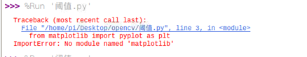
库中没有matplotlib函数,然后我百度了一下,网上一种方法是
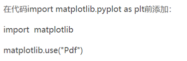
但是还是出现了同样的问题,然后我找到了另一个方法
直接安装: sudo apt-get install python3-matplotlib
ok,成功了,可以运行了

2.自适应阈值
cv2.adaptiveThreshold(src, maxVal, adaptiveMethold, thresholdType, blockSize, C, dst)
src: 原图像,只能输入单通道图像,通常来说为灰度图
maxval: 当像素值超过了阈值(或者小于阈值,根据type来决定),所赋予的值
thresholdType:二值化操作的类型,与固定阈值函数相同,包含5种类型,同上一节。
blockSize: 图片中分块的大小
C :阈值计算方法中的常数项
dst:目标图像
adaptiveMethold: 阈值的计算方法,包含以下2种类型:
cv2.ADAPTIVE_THRESH_MEAN_C, 阈值取自相邻区域的平均值
cv2.ADAPTIVE_THRESH_GAUSSIAN_C, 阈值取值相邻区域的加权和,权重为一个高斯窗口
import cv2
import numpy as np
from matplotlib import pyplot as plt

img = cv2.imread('/home/pi/Desktop/opencv/123.jpg', 0)
img = cv2.medianBlur(img, 5) # 中值滤波

ret, th1 = cv2.threshold(img, 127, 255, cv2.THRESH_BINARY)
# 11 为 Block size, 2 为 C 值
th2 = cv2.adaptiveThreshold(img, 255, cv2.ADAPTIVE_THRESH_MEAN_C, cv2.THRESH_BINARY, 11, 2)
th3 = cv2.adaptiveThreshold(img, 255, cv2.ADAPTIVE_THRESH_GAUSSIAN_C, cv2.THRESH_BINARY, 11, 2)
titles = ['Original Image',
          'Global Thresholding (v = 127)', 'Adaptive Mean Thresholding', 'Adaptive Gaussian Thresholding']
images = [img, th1, th2, th3]
for i in range(4):
    plt.subplot(2, 2, i+1), plt.imshow(images[i], 'gray')
    plt.title(titles[i])
    plt.xticks([]), plt.yticks([])
plt.show()


3.Otsu’s二值化
Otsu’s Binarization是一种基于直方图的二值化方法,它需要和threshold函数配合使用
在第一部分中我们提到过 retVal,当我们使用 Otsu 二值化时会用到它。 那么它到底是什么呢? 在使用全局阈值时,我们就是随便给了一个数来做阈值,那我们怎么知道
我们选取的这个数的好坏呢?答案就是不停的尝试。如果是一副双峰图像(简 单来说双峰图像是指图像直方图中存在两个峰)呢?我们岂不是应该在两个峰之间的峰谷选一个值作为阈值?这就是 Otsu 二值化要做的。简单来说就是对 一副双峰图像自动根据其直方图计算出一个阈值。(对于非双峰图像,这种方法 得到的结果可能会不理想)。 这里用到到的函数还是cv2.threshold(),但是需要多传入一个参数flag:cv2.THRESH_OTSU。这时要把阈值设为 0。然后算法会找到最优阈值,这个最优阈值就是返回值 retVal。如果不使用 Otsu 二值化,返回的 retVal 值与设定的阈值相等。
Otsu过程:
- 计算图像直方图;
- 设定一阈值,把直方图强度大于阈值的像素分成一组,把小于阈值的像素分成另外一组;
- 分别计算两组内的偏移数,并把偏移数相加;
- 把0~255依照顺序多为阈值,重复1-3的步骤,直到得到最小偏移数,其所对应的值即为结果阈值。
import cv2
import numpy as np
from matplotlib import pyplot as plt

img = cv2.imread('/home/pi/Desktop/opencv/123.jpg', 0)
# global thresholding
ret1, th1 = cv2.threshold(img, 127, 255, cv2.THRESH_BINARY)
# Otsu's thresholding
ret2, th2 = cv2.threshold(img, 0, 255, cv2.THRESH_BINARY+cv2.THRESH_OTSU)
# Otsu's thresholding after Gaussian filtering
# (9,9)为高斯核的大小,8 为标准差
blur = cv2.GaussianBlur(img, (9, 9), 8)
# 阈值一定要设为 0!
ret3, th3 = cv2.threshold(blur, 0, 255, cv2.THRESH_BINARY+cv2.THRESH_OTSU)
# plot all the images and their histograms
images = [img, 0, th1, img, 0, th2, blur, 0, th3]
titles = ['Original Noisy Image', 'Histogram', 'Global Thresholding (v=127)', 'Original Noisy Image',
          'Histogram', "Otsu's Thresholding", 'Gaussian filtered Image', 'Histogram', "Otsu's Thresholding"]
# 这里使用了 pyplot 中画直方图的方法,plt.hist, 要注意的是它的参数是一维数组
# 所以这里使用了(numpy)ravel 方法,将多维数组转换成一维,也可以使用 flatten 方法
# ndarray.flat 1-D iterator over an array.
# ndarray.flatten 1-D array copy of the elements of an array in row-major order
for i in range(3):
    plt.subplot(3, 3, i*3+1), plt.imshow(images[i*3], 'gray')
    plt.title(titles[i*3]), plt.xticks([]), plt.yticks([])
    plt.subplot(3, 3, i*3+2), plt.hist(images[i*3].ravel(), 256)
    plt.title(titles[i*3+1]), plt.xticks([]), plt.yticks([])
    plt.subplot(3, 3, i*3+3), plt.imshow(images[i*3+2], 'gray')
    plt.title(titles[i*3+2]), plt.xticks([]), plt.yticks([])
plt.show()

五:平滑图像(图像模糊)
模糊是卷积的一种表现
1.2D卷积

dst=cv.filter2D(src, ddepth, kernel[, dst[, anchor[, delta[, borderType]]]])
src 原图像
dst 目标图像,与原图像尺寸和通过数相同
ddepth 目标图像的所需深度
kernel 卷积核(或相当于相关核),单通道浮点矩阵;如果要将不同的内核应用于不同的通道,请使用拆分将图像拆分为单独的颜色平面,然后单独处理它们。
anchor 内核的锚点,指示内核中过滤点的相对位置;锚应位于内核中;默认值(-1,-1)表示锚位于内核中心。
detal 在将它们存储在dst中之前,将可选值添加到已过滤的像素中。类似于偏置。
borderType 像素外推法
import cv2
import numpy as np
ferom matplotlib import pyplot as plt
img = cv2.imread('/home/pi/Desktop/opencv/123.jpg')
kernel = np.ones((5,5),np.float32)/ 25
dst = cv2.filter2D(img,-1,kernel)
plt.subplot(121),plt.imshow(img),plt.title('Original')
plt.xticks([]),plt.yticks([])
plt.subplot(122),plt.imshow(dst),plt.title('Averaging')
plt.xticks([]),plt.yticks([])
plt.show()

2.均值模糊
import cv2  as  cv
import numpy as np
def blur_demo(image):
     dst = cv.blur(image,(1,15))
     cv.imshow("blur_demo", dst)

print ("--------Hello Python---------")
src =cv.imread("/home/pi/Desktop/opencv/123.jpg")
cv.namedWindow("input image", cv.WINDOW_AUTOSIZE)
cv.imshow("input image", src)
blur_demo(src)
cv.waitKey(0)
cv.destroyAllWindow()

拓展:高斯模糊
import cv2 as cv
import numpy as np


def clamp(pv):
if pv >255:
return 255
if pv <0:
return 0
else:
return pv

def gaussian_noise(image):
h,w,c = image.shape
for row in range(h):
for col in range(w):
s = np.random.normal(0 , 20, 3)
b = image[row, col, 0]
g = image[row, col, 1]
r = image[row, col, 2]
image[row, col, 0] = clamp(b +s[0])
image[row, col, 1] = clamp(g +s[1])
image[row, col, 2] = clamp(r +s[2])
cv.imshow("noise image", image)

print("------Hello Python-------")
src = cv.imread("/home/pi/Desktop/opencv/123.jpg")
cv.namedWindow("input image", cv.WINDOW_AUTOSIZE)
cv.imshow("input image", src)
gaussian_noise(src)
cv.waitKey(0)

cv.destroyAllWindow()

发现有点慢(一开始以为出错了)等了一会就出现了

然后加了一个计算消耗时间的函数

3.中值模糊
import cv2  as  cv
import numpy as np
def median_demo(image):
     dst = cv.medianBlur(image,(1,15))
     cv.imshow("blur_demo", dst)

print ("--------Hello Python---------")
src =cv.imread("/home/pi/Desktop/opencv/123.jpg")
cv.namedWindow("input image", cv.WINDOW_AUTOSIZE)
cv.imshow("input image", src)
median_demo(src)
cv.waitKey(0)
cv.destroyAllWindow()


4.卷积的自定义
import cv2
import numpy as np

def solve():

    src = cv2.imread("./Pictures/car001.jpg")
    if src is None:
        return -1

    kernel = np.array((
        [0, -1 0],
        [-1,5,-1],
        [0,-1,0]), dtype="float32")
改变以上三行的数字实现自定义

    dst = cv2.filter2D(src, -1, kernel)
    htich = np.hstack((src, dst))
    cv2.imwrite("./Pictures/car.jpg", htich)
    cv2.imshow('merged_img', htich)
    cv2.waitKey(0)

    return 0


if __name__ == "__main__":
    solve()

参见: https://www.cnblogs.com/lfri/p/10599420.html