一,卷积神经网络简介
卷积神经网络提供了一种方法来特化神经网络,使其能够处理清楚的网络结构拓扑的数据,以及将这样的模型扩展到非常大的规模。这种方法在二维图像拓扑上是最成功的。
卷积神经网络的主要特征有:
- 稀疏连接:源于视觉的局部感受野。
- 权值共享
- 等变表示:平移等变性。
- 总结:稀疏连接和权值共享降低了参数量,使训练复杂度大大降低,并减轻了过拟合。同时权值共享还赋予了卷积网络对平移的容忍性,而池化层降采样进一步降低了输出餐数量,并赋予模型对轻度形变的容忍性,提高了模型的泛化能力。
卷积神经网络中的一个卷积层一般包括三级:
- 卷积级:利用卷积核加偏置进行仿射变换,提取feature map。
- 探测级:非线性激活函数,如Relu。
- 池化级:降采样,一般用最大池化,保留最显著的特征,并提升模型的畸变容忍能力。
卷积神经网络的参数只与卷积核的大小与数量有关,只要我们提供的卷积核数量足够多,能提取出各种方向的边或者各种形态的点,就可以让卷积层抽象出有效而丰富的高阶特征。
经典卷积网络:
- LeNet5
- AlexNet
- VGG
- GoogleInceptionNet
- ResNet
二,用TensorFlow实现简单的卷积网络
padding的填充方式有三种(假设输入图像宽为m,卷积核宽为k,步长为1):
- valid:无论怎样都不使用零填充的极端情况,并且卷积核只允许访问那些图像中能够完全包含整个核的位置。输出的宽度会变成m-k+1。
- same:只进行足够的零填充来保持输出与输入有相同的大小,这可能会导致边界像素的欠表示。
- full:进行足够的零填充,来保证每个像素在每个方向上正好被访问了k次,最终输出图像的宽度为m+k-1,一般不用。
但,零填充的最优数量处于valid和same padding之间的某个位置。
一些基础
- tf.nn.conv2d(x,filters,strides,padding)
①x=[图像数量(一般为-1代表样本数量不固定),长度,宽度,图像通道数]。
②filters=[长度,宽度,输入图像的通道数,卷积核数]
③strides = [批处理步长(一般为1),长度上的步长,宽度上的步长,卷积核数上的步长(一般为1)]
④padding=’same’或‘valid’,用来定义零填充的方式。 - tf.nn.max_pool(x,pool_kernel,strides,padding)
参数形式同conv2d。
tensorflow的实现
# 一般CNN的实现
import tensorflow as tf
from tensorflow.examples.tutorials.mnist import input_data

# 0,导入数据
mnist = input_data.read_data_sets("MNIST_data/",one_hot=True)
print(mnist.train.images.shape,mnist.train.labels.shape)
sess = tf.InteractiveSession()

# 1,定义一些要重复使用的函数
def weighted_variable(shape):
    initial = tf.truncated_normal(shape,stddev=0.1)
    return tf.Variable(initial)
def bias_variable(shape):
    initial = tf.constant(0.1,shape=shape)
    return tf.Variable(initial)
def conv2d(x,filters):
    return tf.nn.conv2d(x,filters,strides=[1,1,1,1],padding="SAME")
def max_pool_2x2(x):
    return tf.nn.max_pool(x,ksize=[1,2,2,1],strides=[1,2,2,1],padding='SAME')

# 2,定义输入
X = tf.placeholder(tf.float32,[None,784])
y = tf.placeholder(tf.float32,[None,10])
X_image = tf.reshape(X,[-1,28,28,1])

# 3,定义第一个卷积层
W_conv1 = weighted_variable([5,5,1,32])
b_conv1 = bias_variable([32])
h_conv1 = tf.nn.relu(conv2d(X_image,W_conv1)+b_conv1)
h_pool1 = max_pool_2x2(h_conv1)

# 4,定义第二个卷积层
W_conv2 = weighted_variable([5,5,32,64])
b_conv2 = bias_variable([64])
h_conv2 = tf.nn.relu(conv2d(h_pool1,W_conv2)+b_conv2)
h_pool2 = max_pool_2x2(h_conv2)

# 5,定义全连接层
W_fc1 = weighted_variable([7*7*64,1024])
b_fc1 = bias_variable([1024])
h_pool2_flat = tf.reshape(h_pool2,[-1,7*7*64])
h_fc1 = tf.nn.relu(tf.matmul(h_pool2_flat,W_fc1)+b_fc1)

# 6,定义dropout层和输出层
keep_prob = tf.placeholder(tf.float32)
h_fc1_dropout = tf.nn.dropout(h_fc1,keep_prob)
W_fc2 = weighted_variable([1024,10])
b_fc2 = bias_variable([10])
y_pred = tf.nn.softmax(tf.matmul(h_fc1_dropout,W_fc2)+b_fc2)

# 7,定义损失函数和优化器
cross_entropy = tf.reduce_mean(-tf.reduce_sum(y*tf.log(y_pred),reduction_indices=[1]))
train_step = tf.train.AdamOptimizer(1e-4).minimize(cross_entropy)

# 8,定义评测准确率的操作
correct_prediction = tf.equal(tf.argmax(y_pred,1),tf.argmax(y,1))
accuracy = tf.reduce_mean(tf.cast(correct_prediction,tf.float32))

# 9,迭代训练
tf.global_variables_initializer().run()
epoch_num = 1
for epoch in range(epoch_num):
    avg_accuracy = 0.0
    avg_cost = 0.0
    for i in range(20000):
        batch_xs,batch_ys = mnist.train.next_batch(50)
        if i%100==0:
            train_accuracy = accuracy.eval(feed_dict={X:batch_xs,y:batch_ys,keep_prob:1.0})
            print("step %d,train accuracy is %.4f"%(i,train_accuracy))
        train_step.run(feed_dict={X:batch_xs,y:batch_ys,keep_prob:0.5})
print('Train Finished!')
print('Test accuracy is %.4f.' % accuracy.eval({X: mnist.test.images, y: mnist.test.labels, keep_prob: 1.0}))

# last,Get one and predict
import matplotlib.pyplot as plt
import random
r = random.randint(0, mnist.test.num_examples - 1)
print("Label:", sess.run(tf.argmax(mnist.test.labels[r:r+1], 1)))
print("Prediction:", sess.run(tf.argmax(y_pred, 1),feed_dict={X: mnist.test.images[r:r + 1],keep_prob:1.0}))
plt.imshow(mnist.test.images[r:r + 1].reshape(28, 28), cmap='Greys', interpolation='nearest')
plt.show()

sess.close()
最后得到的准确率约为99.2%。
三,用TensorFlow实现高级的卷积网络
此次分类的数据集使用了CIFAR-10,而不是Mnist。
使用的一些新的技巧:
扫描二维码关注公众号,回复:
1004033 查看本文章

- 对weights进行L2正则化。
- 对图片进行了翻转、随机剪切等数据增强,制造了更多样本。
- 在每个卷积-最大池化层后面使用了LRN层(局部响应归一化层),增强了模型的泛化能力。
LRN层模拟了生物神经系统的侧抑制机制,对局部神经元的活动创建竞争环境,使得其中响应比较大的值变得相对更大,并抑制其他反馈较小的神经元,增强了模型的泛化能力。LRN对ReLU这种没有上限边界的激活函数会比较有用,因为它会从附近多个卷积核的响应中选择比较大的反馈,但不适合Sigmoid这种有固定边界并且能抑制过大值的激活函数。
一些基础
- tf.nn.l2_loss(w1):求w1的L2正则化项的损失;
- cifar10_input.distorted_inputs(data_dir,batch_size):这个函数包含了数据增强的各种操作:tf.image.random_flip_left_right、tf.random_crop、tf.image.random_brightness、tf.image.random_contrast和数据标准化tf.image.per_image_whitening。
- tf.add_to_collection(name,var):将var放到名为name的collection里;
- tf.get_collection(name):取回名为name的collection里的内容;
- tf.nn.lrn(pool1,4,bias=1.0,alpha=0.001/9.0,beta=0.75):LRN层;
- tf.nn.sparse_softmax_cross_entropy_with_logits(logits=logits,labels=labels,name=’cross_entropy_per_example’):先对logits进行softmax,再计算和整数表示的label的交叉熵。
- tf.nn.in_top_k(logits,labels,1):输出结果中top k的准确率,默认使用top 1。
- tf.train.start_queue_runners():添加线程队列,来对某些操作进行加速,这里是对数据增强的那些操作进行加速。
tensorflow的实现
import cifar10,cifar10_input
import tensorflow as tf
import numpy as np
import time

max_steps = 3000
batch_size = 128
data_dir = '/tmp/cifar10_data/cifar-10-batches-bin'


def variable_with_weight_loss(shape, stddev, wl):
    var = tf.Variable(tf.truncated_normal(shape, stddev=stddev))
    if wl is not None:
        weight_loss = tf.multiply(tf.nn.l2_loss(var), wl, name='weight_loss')
        tf.add_to_collection('losses', weight_loss)
    return var
def loss(logits, labels):
    #      """Add L2Loss to all the trainable variables.
    #      Add summary for "Loss" and "Loss/avg".
    #      Args:
    #        logits: Logits from inference().
    #        labels: Labels from distorted_inputs or inputs(). 1-D tensor
    #                of shape [batch_size]
    #      Returns:
    #        Loss tensor of type float.
    #      """
    #      # Calculate the average cross entropy loss across the batch.
    labels = tf.cast(labels, tf.int64)
    # sparse_Softmax_cross_entropy_with_logits:中logits中的元素是向量形式而labels的元素是整数,所以是sparseD的
    cross_entropy = tf.nn.sparse_softmax_cross_entropy_with_logits(
        logits=logits, labels=labels, name='cross_entropy_per_example')
    cross_entropy_mean = tf.reduce_mean(cross_entropy, name='cross_entropy')
    tf.add_to_collection('losses', cross_entropy_mean)

    # The total loss is defined as the cross entropy loss plus all of the weight
    # decay terms (L2 loss).
    return tf.add_n(tf.get_collection('losses'), name='total_loss')


###

cifar10.maybe_download_and_extract()

images_train, labels_train = cifar10_input.distorted_inputs(data_dir=data_dir,
                                                            batch_size=batch_size)

images_test, labels_test = cifar10_input.inputs(eval_data=True,
                                                data_dir=data_dir,
                                                batch_size=batch_size)
# images_train, labels_train = cifar10.distorted_inputs()
# images_test, labels_test = cifar10.inputs(eval_data=True)

image_holder = tf.placeholder(tf.float32, [batch_size, 24, 24, 3])
label_holder = tf.placeholder(tf.int32, [batch_size])

# logits = inference(image_holder)

# 1,第一层:卷积+ReLU+最大池化+LRN
weight1 = variable_with_weight_loss(shape=[5, 5, 3, 64], stddev=5e-2, wl=0.0)
kernel1 = tf.nn.conv2d(image_holder, weight1, [1, 1, 1, 1], padding='SAME')
bias1 = tf.Variable(tf.constant(0.0, shape=[64]))
conv1 = tf.nn.relu(tf.nn.bias_add(kernel1, bias1))
pool1 = tf.nn.max_pool(conv1, ksize=[1, 3, 3, 1], strides=[1, 2, 2, 1],
                       padding='SAME')
norm1 = tf.nn.lrn(pool1, 4, bias=1.0, alpha=0.001 / 9.0, beta=0.75)

# 2,第二层:卷积+ReLU+LRN+最大池化
weight2 = variable_with_weight_loss(shape=[5, 5, 64, 64], stddev=5e-2, wl=0.0)
kernel2 = tf.nn.conv2d(norm1, weight2, [1, 1, 1, 1], padding='SAME')
bias2 = tf.Variable(tf.constant(0.1, shape=[64]))
conv2 = tf.nn.relu(tf.nn.bias_add(kernel2, bias2))
norm2 = tf.nn.lrn(conv2, 4, bias=1.0, alpha=0.001 / 9.0, beta=0.75)
pool2 = tf.nn.max_pool(norm2, ksize=[1, 3, 3, 1], strides=[1, 2, 2, 1],
                       padding='SAME')

# 3,第三层:全连接层(ReLU)
reshape = tf.reshape(pool2, [batch_size, -1])
dim = reshape.get_shape()[1].value
weight3 = variable_with_weight_loss(shape=[dim, 384], stddev=0.04, wl=0.004)
bias3 = tf.Variable(tf.constant(0.1, shape=[384]))
local3 = tf.nn.relu(tf.matmul(reshape, weight3) + bias3)

# 4,第四层:全连接层(ReLU)
weight4 = variable_with_weight_loss(shape=[384, 192], stddev=0.04, wl=0.004)
bias4 = tf.Variable(tf.constant(0.1, shape=[192]))
local4 = tf.nn.relu(tf.matmul(local3, weight4) + bias4)

# 5,第五层:全连接层
weight5 = variable_with_weight_loss(shape=[192, 10], stddev=1 / 192.0, wl=0.0)
bias5 = tf.Variable(tf.constant(0.0, shape=[10]))
logits = tf.add(tf.matmul(local4, weight5), bias5)

loss = loss(logits, label_holder)

train_op = tf.train.AdamOptimizer(1e-3).minimize(loss)  # 0.72

top_k_op = tf.nn.in_top_k(logits, label_holder, 1)

sess = tf.InteractiveSession()
tf.global_variables_initializer().run()

# 启动前面提到的数据增强的线程队列,16个线程进行加速
tf.train.start_queue_runners()
###
for step in range(max_steps):
    start_time = time.time()
    image_batch, label_batch = sess.run([images_train, labels_train])
    _, loss_value = sess.run([train_op, loss], feed_dict={image_holder: image_batch,
                                                          label_holder: label_batch})
    duration = time.time() - start_time

    if step % 10 == 0:
        examples_per_sec = batch_size / duration
        sec_per_batch = float(duration)

        format_str = ('step %d, loss = %.2f (%.1f examples/sec; %.3f sec/batch)')
        print(format_str % (step, loss_value, examples_per_sec, sec_per_batch))

###
num_examples = 10000
import math

num_iter = int(math.ceil(num_examples / batch_size))
true_count = 0
total_sample_count = num_iter * batch_size
step = 0
while step < num_iter:
    image_batch, label_batch = sess.run([images_test, labels_test])
    predictions = sess.run([top_k_op], feed_dict={image_holder: image_batch,
                                                  label_holder: label_batch})
    true_count += np.sum(predictions)
    step += 1

precision = true_count / total_sample_count
print('precision @ 1 = %.3f' % precision)
结果
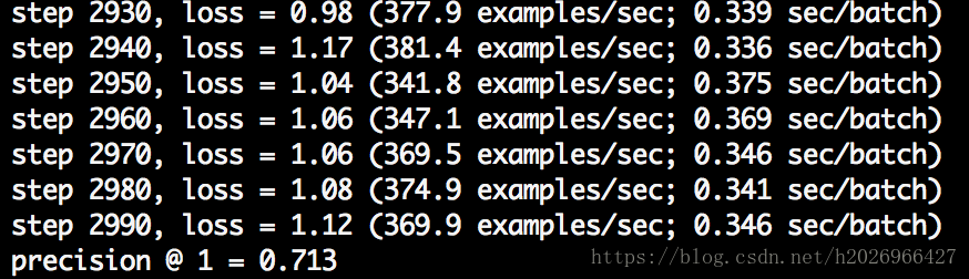
增大max_steps、使用学习速率衰减的SGD进行训练,会使准确率进一步上升,大致接近86%。