Article directory
1. Two-dimensional data curve chart
1.1. Drawing a single two-dimensional curve
1.2. Drawing of multiple two-dimensional curves
1.4. Graphic annotation and coordinate control
1.5. Adaptive sampling drawing
1.6. Division of graphics window
2. Drawing of other two-dimensional graphics
Preface
After the previous period of study, I have become proficient in using MATLAB for programming and numerical calculations. However, numerical calculations are discrete data after all. No matter how perfect and accurate it is, it is still difficult for us to directly calculate it from Feel their specific meaning and inherent laws from a large amount of data. People prefer to intuitively feel the global significance and many inner essences of scientific calculation results through graphics, so they have to use another function of MATLAB, the powerful graphics drawing capability.
MATLAB has powerful graphics expression functions. It can draw not only two-dimensional graphics, but also three-dimensional graphics. It can also modify graphics through operations such as annotation, viewpoint, color, and lighting. MATLAB has two types of drawing commands, one is the low-level drawing commands that directly operate on the graphics handle, and the other is the high-level drawing commands built on the low-level commands. We mainly learn high-level drawing commands, which are simple, clear, convenient and efficient.
1. Two-dimensional data curve chart
A two-dimensional data graph is a plane graph that connects data points on plane coordinates. Different coordinate systems can be used. In addition to the rectangular coordinate system, logarithmic coordinates, polar coordinates, etc. can also be used. Data points can be given in vector or matrix form, and the type can be real or complex.
1.1. Drawing a single two-dimensional curve
In MATLAB, the plot function can be used to draw a two-dimensional curve in a rectangular coordinate system, which is widely used.
The calling format of plot function is:
plot(x,y)
Among them, x and y are vectors with the same length, used to store x coordinate and y coordinate data respectively. The plot function is used to draw two-dimensional curves with x as the abscissa and y as the ordinate, respectively. y(i) is the function value of the x(i) point.

1.2. Drawing of multiple two-dimensional curves
1. The input parameters of the plot function are in matrix form:
When the input parameter of the plot function is a vector, a single curve is drawn. This is the most basic usage. But in actual applications, the input parameters of the plot function can be in matrix form, in which case multiple curves will be drawn in the same coordinate system with different colors.
① When x is a vector and y is a matrix with one dimension and the same dimension as x, multiple curves of different colors are drawn. The number of curves is equal to the other dimension of the y matrix, and x is used as the common abscissa of these curves. .
② When x and y are matrices of the same dimension, use the corresponding column elements of x and y as the horizontal and vertical coordinates to draw curves respectively. The number of curves is equal to the number of columns of the matrix.
③ For the plot function that contains only one input parameter, when the input parameter is a real matrix, the curve of the element value of each column relative to its subscript is drawn column by column. The number of curves is equal to the number of columns of the input parameter matrix.
2. Plot function with multiple input parameters
The plot function can contain several sets of vector pairs, and each vector pair can draw a curve.
The calling format of plot function with multiple input parameters is:
plot(x1,y1,x2,y2,x3,y3,......xn,yn)
① When the input parameters are all vectors, x1, y1, x2 and y2 form a set of vector pairs respectively. The length of each set of vector pairs can be different. Each set of vector pairs can draw a curve, so that at the same coordinate Multiple curves are drawn in the system.
② When the input parameter has a matrix, the paired x and y curves are drawn according to the horizontal and vertical coordinates of the corresponding column elements. The number of curves is equal to the number of columns of the matrix.
3. Graphic retention
Under normal circumstances, the MATLAB drawing command refreshes the current graphics window every time it is executed, and the original graphics in the graphics window no longer exist. If you want to continue to add new graphics to the existing graphics, you can use the graphics hold command hold. The hold on command maintains the original graphics, and the hold off command refreshes the original graphics.

1.3. Set curve style
When we draw multiple curves in MATLAB, in order to better distinguish the curves, the color and type of the curves is a good way. MATLAB provides some drawing options for the color of the curve and the style of the curve, as shown in the following table:
① Curve line type options:
| symbol |
linear |
symbol |
linear |
| - |
Solid line (default) |
-. |
Dotted line |
| : |
dotted line |
-- |
double dash |
② Curve color options:
| symbol |
color |
symbol |
color |
| b (blue) |
blue |
m (magenta) |
magenta |
| g (green) |
green |
y (yellow) |
yellow |
| r (red) |
red |
k (black) |
black |
| c (cyan) |
blue |
w (white) |
white |
③ Mark symbol options:
| Options |
mark symbol |
Options |
mark symbol |
| . |
point |
∨ |
downward facing triangle symbol |
| O (letter) |
circle |
∧ |
upward triangle symbol |
| X (letter) |
Cross |
< |
Left facing triangle symbol |
| + |
plus |
> |
right facing triangle symbol |
| * |
Asterisk |
p (pentagram) |
pentagram symbol |
| s (square) |
Square symbol |
h (hexagram) |
six pointed star symbol |
| d (diamond) |
rhombus talisman |
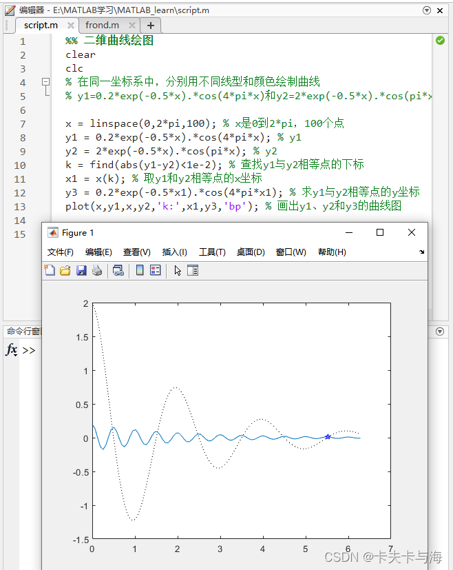
As shown in the figure above, curve y1 is the default value (i.e., blue solid line), curve y2 is a black dotted line, and the place where curves y1 and y2 intersect (the x values are equal) is marked with a blue five-pointed star symbol. When such a curve is displayed in the same coordinate system, we can see it clearly at a glance.
1.4. Graphic annotation and coordinate control
1. Graphic annotation:
While drawing a graph, you can add some descriptions to the graph, such as the name of the graph, description of the coordinate axis, and the meaning of a certain part of the graph. These operations are called adding graph annotations to make the meaning of the graph clearer and more readable.
The calling format of the graphic annotation function is:
① title (graph name)
② ylabel (y-axis description)
③ xlabel (x-axis description)
④ zlabel (z-axis description)
⑤ text(x, y, graphic description)
⑥ legend(Legend 1, Legend 2,...)
The title and xlabel, ylabel, and zlabel functions are used to describe the names of graphics and coordinate axes respectively. The text function adds a graphic description at the (x, y) coordinates. The legend function is used to mark the legend with the line type, color or data points used to draw the curve. The legend is placed in the blank space of the graph and can also be moved with the mouse.
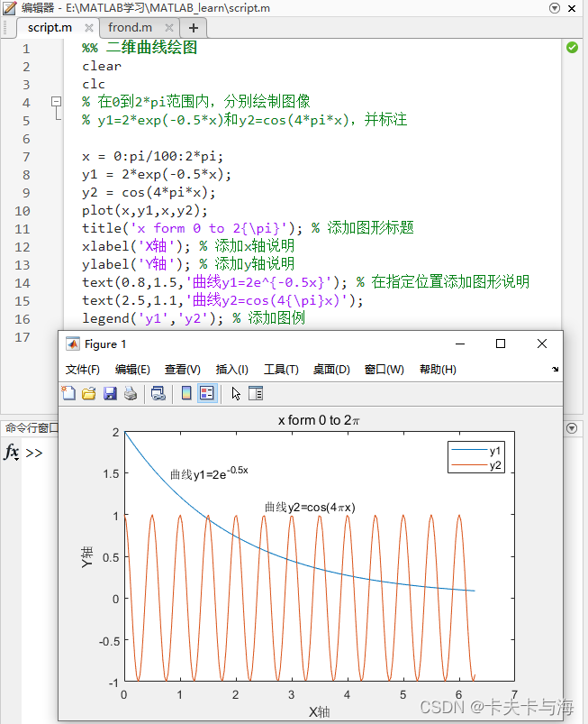
As shown in the figure above, when drawing the graph, we added a graph description, as well as a coordinate axis description and a curve description, so that we can know which function the two curves are respectively, and it is also helpful for us to do mathematical analysis.
2. Coordinate control
When we draw graphics, MATLAB can automatically select the appropriate coordinate scale based on the range of the curve data to be drawn, so that the curve can be displayed as clearly as possible, so generally there is no need to consider the scale range of the coordinates. If the user needs to select the scale range of coordinates under special circumstances, it can be set using the axis function. The calling format of this function is: axis([xmin xmax ymin ymax zmin zmax]). Its parameters are the minimum and maximum values of the x-axis, y-axis and z-axis respectively. In addition, the axis function has many functions. Commonly used formats are:
Common formats for axis functions:
① axis equal: The vertical and horizontal axes adopt equal length scales
② axis square: generates a square coordinate system (default is rectangular)
③ axis auto: use default settings
④ axis off: Cancel the coordinate system
⑤ axis on: display coordinate system
In addition to the above functions used to set the display range of coordinates, you can also add grid lines to coordinates, which are controlled by the grid command. The grid on/off command controls whether to draw grid lines; adding borders to coordinates can be controlled by the box command. , the box on/off command controls whether to add a border to the coordinates.
1.5. Adaptive sampling drawing
Earlier we learned the plot drawing function. The basic principle of this function is to first take a sufficiently dense independent variable vector x, then calculate the function value vector y, and finally use the drawing function to draw. The function graph drawn in this way is sampled at equal intervals, only Suitable for situations where accuracy requirements are not high. However, if the accuracy of the curve is very high, the method of sampling at equal intervals is not feasible. In this case, intensive sampling is needed in the section with a large change rate to fully reflect the actual change pattern of the function, and the fplot function is This function can be realized well and the authenticity of graphics can be improved.
The calling format of fplot function is:
fplot(@(argument)fname,lims,options)
Among them, the @() brackets contain independent variables, such as @(x). fname is the function name, which appears in the form of a string; lims is the value range of x and y, which appears in the form of a row vector; the options are set to the curve color, Style etc.
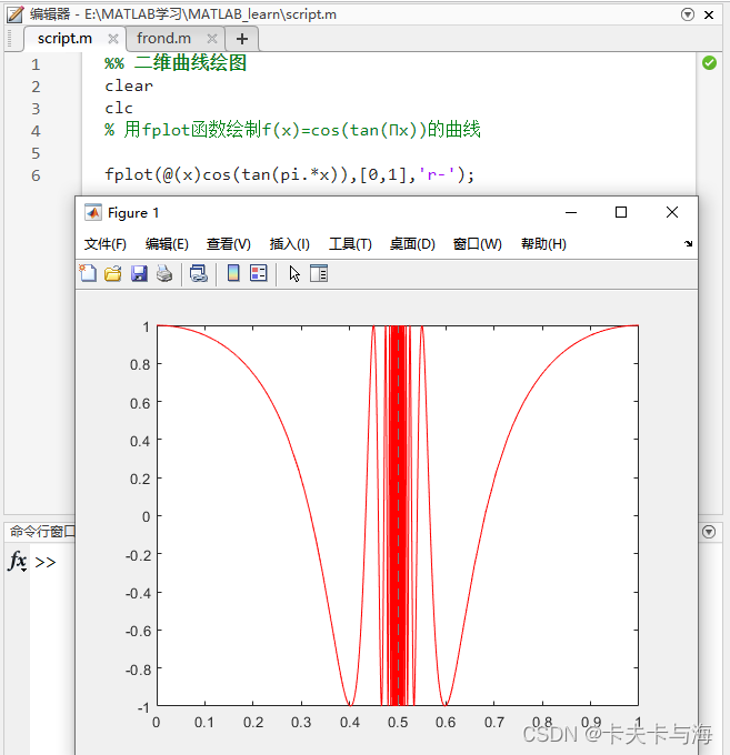
As shown in the figure above, it is a graph drawn by the fplot function. The independent variable is x, the function name is cos(tan(pi*x)), the display range is 0 to 1, and the option type is drawn with a red horizontal line.
1.6. Division of graphics window
In practical applications, it is often necessary to draw several independent graphics in a graphics window. In this case, the graphics window needs to be divided. The divided graphics window will display several drawing areas. Each drawing area can establish an independent coordinate system and draw graphics. In graphics window division, MATLAB provides the subplot function, whose calling format is: subplot(m,n,p). This function divides the current graphics window into m*n drawing areas, where p represents the current drawing area.

2. Drawing of other two-dimensional graphics
Earlier we talked about two-dimensional graphics drawing in the rectangular coordinate system, but in addition to using the rectangular coordinate system, two-dimensional graphics can also use the logarithmic coordinate system or polar coordinate system, etc. Let's learn about the logarithmic coordinate system or polar coordinate system together. Draw the two-dimensional data curve under the coordinate system!
① Logarithmic coordinate system drawing:
semilogx(x1,y1,option1,x2,y2,option2,...)
semilogy(x1,y1,option 1,x2,y2,option 2,...)
loglog(x1,y1,option1,x2,y2,option2,...)
The definition of the options is exactly the same as that of the plot function. The difference is the selection of the coordinate axis; the semilogx function uses semi-logarithmic coordinates, the x-axis is a commonly used logarithmic scale, and the y-axis maintains a linear scale; semilogy also uses a semi-logarithmic coordinate system. , the y-axis is a commonly used logarithmic scale, while the x-axis maintains a linear scale; the loglog function uses a fully logarithmic coordinate system, and both the x and y axes use commonly used logarithmic scales.
② Polar coordinate system drawing:
polar(theta,rho,option)
Among them, theta is the polar angle in polar coordinates, rho is the vector radius in polar coordinates, and the content of the options is the same as the plot function.
③ bar(x,y,option): Bar chart
④ stairs(x,y,option): ladder diagram
⑤ stem(x,y,option): rod graph
⑥ fill(x1,y1,option 1,x2,y2,option 2,...)

Summarize
That’s it for today’s MATLAB study. This time I learned about two-dimensional graphics drawing, including two-dimensional graphics drawing in the rectangular coordinate system and other coordinate systems. I also learned the labeling of graphics, the display range of graphics, etc. Among them, in the direct coordinate system Two-dimensional graphics drawing is something we often use, and we can use more examples to deepen our impression.