MATLAB graphics drawing-polar and logarithmic images

Polar and logarithmic images

Polar coordinate image:

If you have studied advanced mathematics, you will definitely not be unfamiliar with the calculus inside, and the images inside will not be unfamiliar. Recall that when we draw these strange images with our hands, we can actually MATLABdraw them easily. Let's take a look at the polar coordinate image. Its parameters include polar diameter rand polar angle. theta
As the first example, we draw a simple curve: Archimedes spiral,

which ais a constant. We draw a polar coordinate image between a = 2and angle. In the 0～2*pifirst statement, we define a constant:

a = 2;

Then we define the function r, which needs to be completed in two steps. In the first step, we treat the angle as a variable and define its interval length and increment:

>> theta = [0:pi/90;2*pi];

Then we write the function:

>> r = a*theta;

Then we draw the image:

In the second example, suppose we draw the following polar coordinate image:
the angle range here is 0～6*pidrawn with a dotted line.
First we define the angle interval:

>> theta = [0:pi/90:6*pi];

Input function:

>> r = 1 + 2*cos(theta);

We tell MATLABto draw with a red dotted line:

>> polar(theta,r,'r-.')

image:

Logarithmic image:

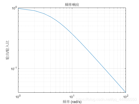
Now let's see MATLABhow to draw a logarithmic image. This used to give me a headache. If you are an electronic engineer, you will find this feature very useful. The first logarithmic image we can use is an log-logimage. We use a very classic example in an electronic circuit to see how to use it. This circuit contains a voltage source, capacitance and resistance. Since many readers are not electronic engineers, we do not need to discuss the source of this formula. Our purpose is only one: How to get a logarithmic image
It turns out that if the input voltage satisfies the sine relationship:

then the output voltage will be another sine function:

where the response frequency, which is the ratio of output to input (magnification), they have the following relationship:

general The frequency response tells us how much the output signal enhances the input signal at different frequencies. We can use it 拉普拉斯变换, so we can make

We take wthe range 1～100between, the unit of the product of resistance Rand capacitance is seconds. For our example, let seconds. These quantities are defined below :CRCRC = 0.25MATLAB

>> RC = 0.25;
>>s = [1:100]*i;

Note that in the second line, we sdefine complex variables. Frequency response is a logarithmic relationship between output / input and frequency, so we define:

So we pass the function to:

>> F = abs(1./(1+RC*s));

Now that all the conditions are there, the same plotcommand can be loglogused in:

>> loglog(imag(s),F),grid on,xlabel('频率 (rad/s)'),ylabel('输出/输入比'),title('频率响应')

This produces a very beautiful image:

Another case of using logarithmic images:

log-logAnother type of image that uses images is when the given function transforms very quickly within a small range of the domain.
Let's look at an example of a function, xthe scope of which is 0～20between:

we first use ordinary methods to draw images:

>> x = [0:0.01:20];
>> y = exp(-10*x.^2);
>> plot(x,y),grid on

We can see that everything happened within a small range of the data set, let's try logarithmic images:

>> loglog(x,y)

Our xaxes and yaxes are in logarithmic form, we can also let them use 1，2，3such direct values ​​directly, then we need the following two commands

• semilogx(x,y): The image xaxis it produces uses logarithmic values, while the yaxis uses direct values
• semilogy(x,y): The image yaxis it produces uses logarithmic values, while the xaxis uses direct values